Split ring commutator? More like split ring commuHATER!

Students find learning about electric motors difficult because:

  1. They find it hard to predict the direction of the force produced on a conductor in a magnetic field, either with or without Fleming’s Left Hand Rule.
  2. They find it hard to understand how a split ring commutator works.

In this post, I want to focus on a suggested teaching sequence for the action of a split ring commutator, since I’ve covered the first point in previous posts.

Who needs a ‘split ring commutator’ anyway?

We all do, if we are going to build electric motors that produce a continuous turning motion.

If we naively connected the ends of a coil to power supply, then the coil would make a partial turn and then lock in place, as shown below. When the coil is in the vertical position, then neither of the Fleming’s Left Hand Rule (FLHR) forces will produce a turning moment around the axis of rotation.

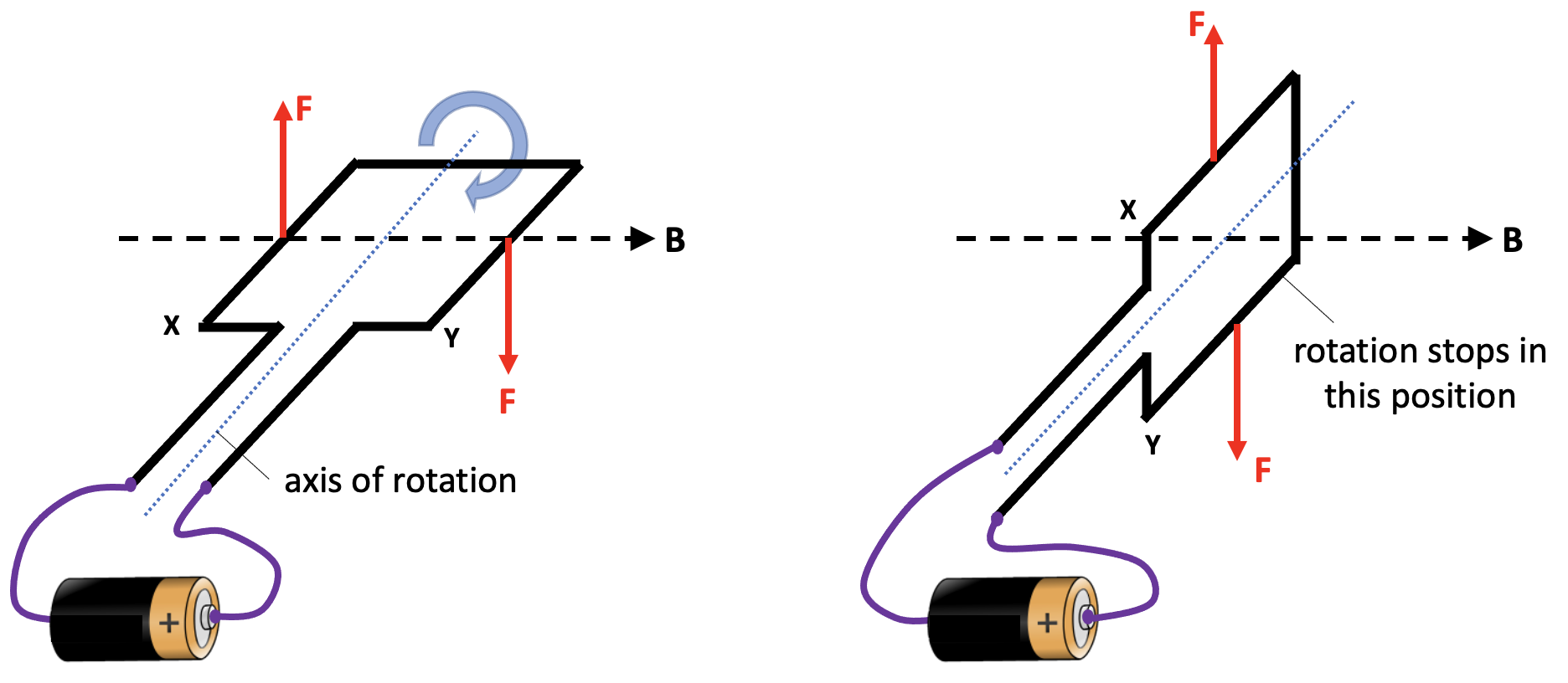
When the coil moves into this vertical position, two things would need to happen in order to keep the coil rotating continuously in the same direction.

  • The current to the coil needs to be stopped at this point, because the FLHR forces acting at this moment would tend to hold the coil stationary in a vertical position. If the current was cut at this time, then the momentum of the moving coil would tend to keep it moving past this ‘sticking point’.
  • The direction of the current needs to be reversed at this point so that we get a downward FLHR force acting on side X and an upward FLHR force acting on side Y. This combination of forces would keep the coil rotating clockwise.

This sounds like a tall order, but a little device known as a split ring commutator can help here.

One (split) ring to rotate them all

The word commutator shares the same root as commute and comes from the Latin commutare (‘com-‘ = all and ‘-mutare‘ = change) and essentially means ‘everything changes’. In the 1840s it was adopted as the name for an apparatus that ‘reverses the direction of electrical current from a battery without changing the arrangement of the conductors’.

In the context of this post, commutator refers to a rotary switch that periodically reverses the current between the coil and the external circuit. This rotary switch takes the form of a conductive ring with two gaps: hence split ring.

Tracking the rotation of a coil through a whole rotation

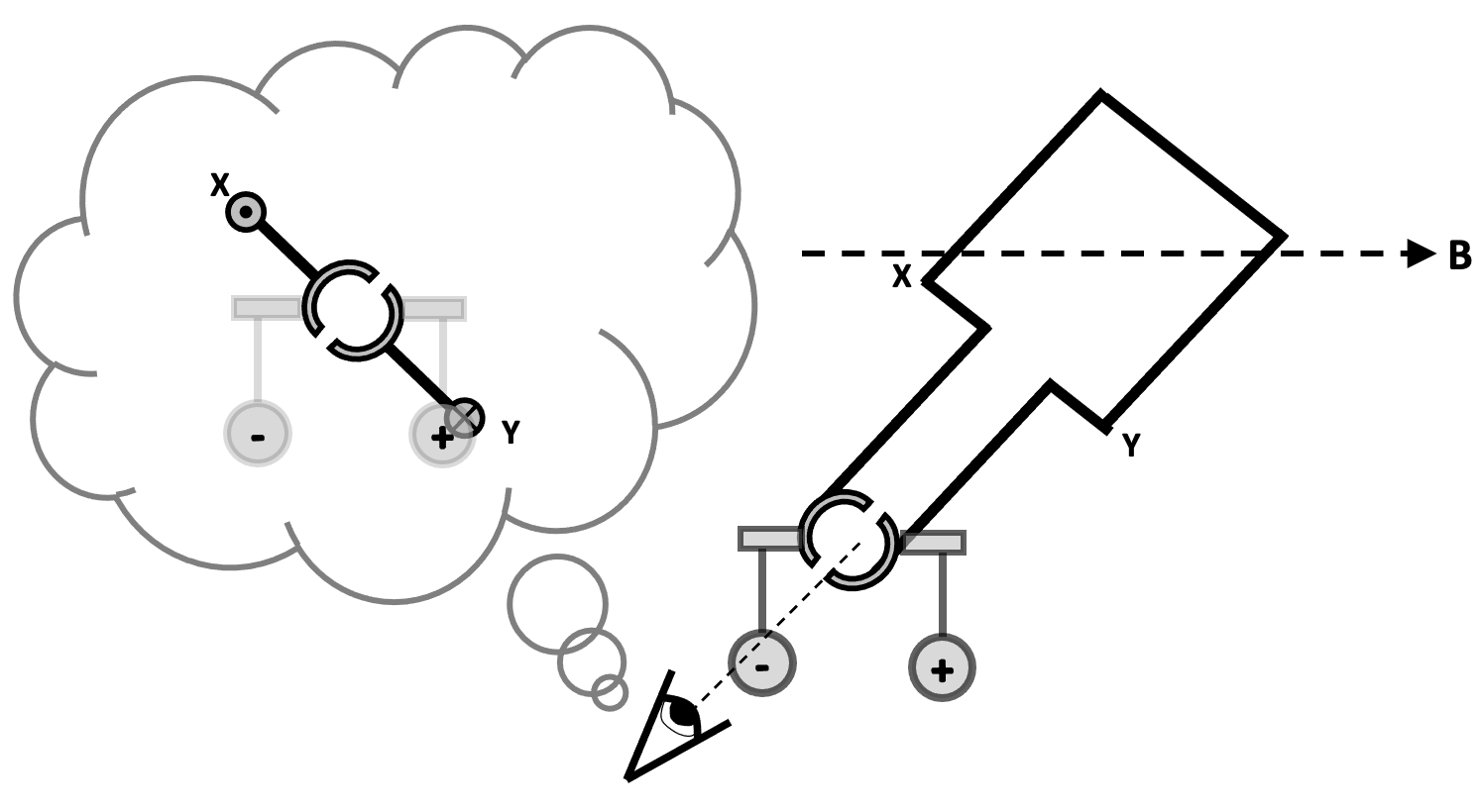
In this picture below, we show the coil connected to a dc power supply via two ‘brushes’ which rest against the split ring commutator (SRC). Current is flowing towards us through side X of the coil and away from us through side Y of the coil (as shown by the dot and cross 2D version of the diagram. This produces an upward FLHR force on side X and a downward FLHR force on side Y which makes the coil rotate clockwise.

Now let’s look at the coil when it has turned 45 degrees. We note that the SRC has also turned by 45 degrees. However, it is still in contact with the brushes that supply the current. The forces on side X and side Y are as noted before so the coil continues to turn clockwise.

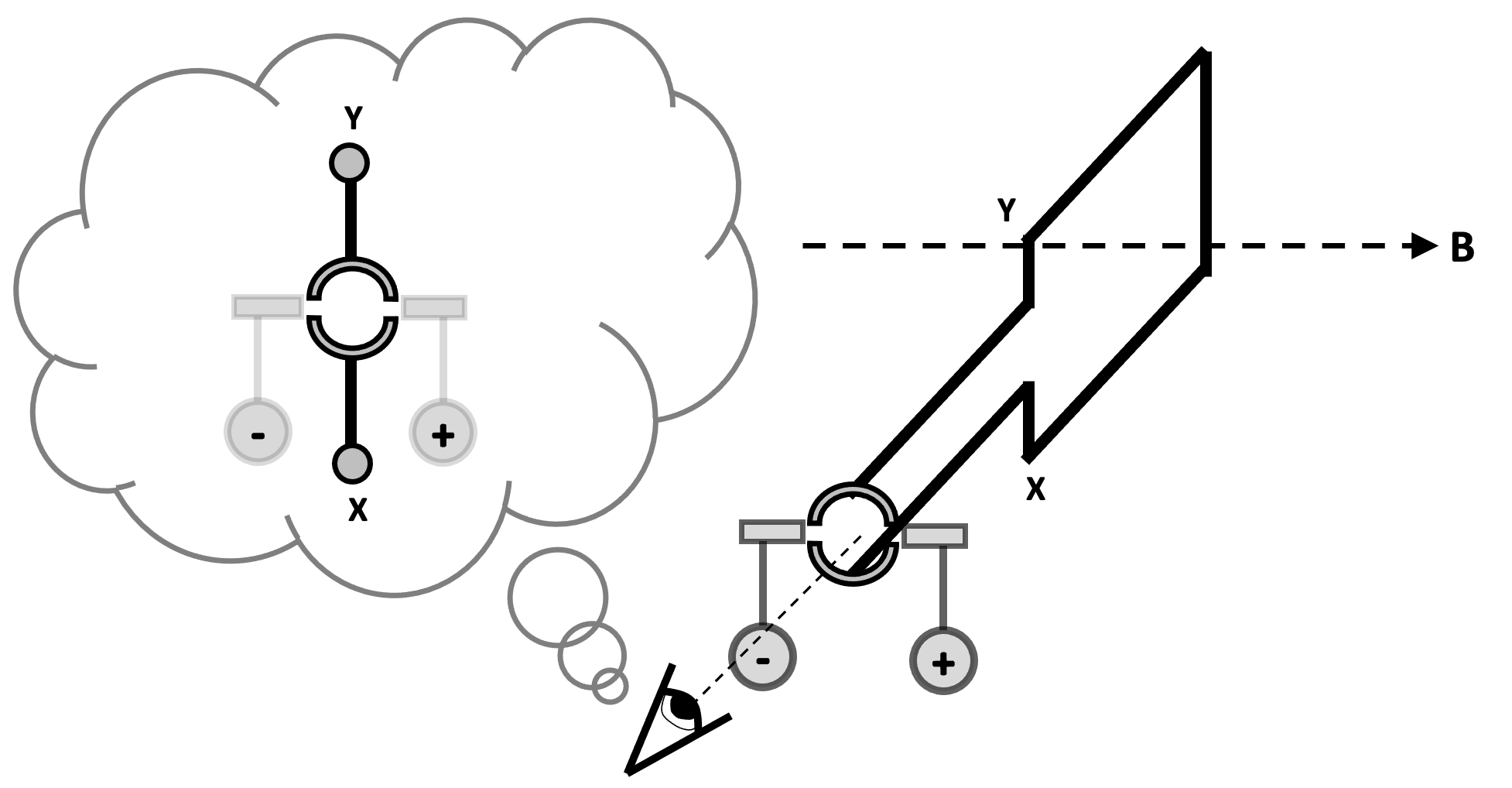
Next, we look at the situation when the coil has turned by another 45 degrees. The coil is now in a vertical position. However, we see that the gaps in the SRC are now opposite the brushes. This means that no current is being supplied to the coil at this point, so there are no FLHR forces acting on sides X and side Y. The coil is free to continue rotating clockwise because of momentum.

Let’s now look at the situation when the coil has rotated a further 45 degrees to the orientation shown below. Note that the side of the SRC connected to X is now touching the brush connected to the positive side of the power supply. This means that current is now flowing away from us through side X (whereas previously it was flowing towards us). The current has reversed direction. This creates a downward FLHR force on side X and an upward FLHR force on side Y (since the current in Y has also reversed direction).

And a short time later when the coil has moved a total of180 degrees from its starting point, we can observe:

And later:

And later still:

And then:

And then eventually we get back to:

Summary

In short, a split ring commutator is a rotary switch in a dc electric motor that reverses the current direction through the coil each half turn to keep it rotating continuously.

A powerpoint of the images used is here:

And a worksheet that students can annotate (and draw the 2D versions of the diagrams!) is here:

I hope that this teaching sequence will allow more students to be comfortable with the concept of a split ring commutator — anything that results in a fewer split ring commuHATERS would be a win for me 😉

Whoa, black body (bam-ba-lam): part two

In part one, we looked at the fact that the hotter an object then the greater the intensity of electromagnetic radiation that will be emitted. For simplicity, we looked at so-called ‘blackbodies’ — that is say, objects which are perfect absorbers (hence ‘blackbodies’) and more importantly, perfect emitters of electromagnetic radiation.

To human eyes, things look very dull in the visible part of the electromagnetic spectrum until we reach temperatures of several hundreds of degrees — however, objects at room temperature (or just above) glow brightly in the infrared part of the electromagnetic spectrum, as we can see easily if we have access to an infrared camera.

By ‘intensity’ of course, we mean the power (‘energy per second’) emitted per unit area.

This links in neatly with 4.6.3.2 of the 2015 AQA GCSE Physics specification:

Stretch and challenge for students (1): Is the intensity of emitted radiation directly proportional to the temperature of the object?

The short answer is no. If you doubled the temperature (measured in kelvins!) of an object then the intensity of radiation would increase by a factor of 16. In other words, the intensity I of radiation emitted by an object is directly proportional to the absolute temperature T raised to the power of 4.

This is a consequence of the Stefan-Boltzmann radiation law (covered in A-level Physics):

In part 1 we estimated the intensity of radiation emitted by two blackbodies by ‘counting squares’ to find the area underneath a graph. We can show that the values obtained are consistent with the Stefan-Boltzmann radiation law.

Since we have dealt comprehensively with the relationship between intensity of radiation and temperature, I propose to move along and look at how the wavelength distribution changes with the temperature of the body.

How does the temperature of a blackbody affect the distribution of emitted wavelengths?

Let’s consider an object that approximates to a blackbody: the filament of an old school incandescent lamp.

The graph of the radiation produced by both objects is shown below.

First, let’s look at the visible wavelengths produced by both bulbs.

  • The 1700 degree Celsius bulb produces only a very small amount of visible light and the vast majority of that is towards the red end of the spectrum: you can see the section where the left hand edge of the 1700 curve just nicks the visible light wavelengths. This means that the 1700 degree filament emits a barely perceptible reddish glow to our eyes with its peak output still firmly in the infrared.
  • The 2200 degree Celsius bulb produces a much larger amount of visible light: look at the left hand side of the curve. What is more, it appears as white light to our eyes since it includes all the colours of the rainbow. However, it’s still a very reddish-tinged white. Photographs taken in artificial light with chemical films (very old school!) had to be taken using special colour balanced film stock otherwise this bias was very evident in the final print(!) Modern digital cameras have software that automatically compensates for artificial vs. daylight colour balance issues.

Second, let’s look at the position of the peak wavelength.

  • The 1700 degree Celsius bulb has its peak output at a wavelength of 1.5 x 10⁻⁶ m (shown by the blue dotted line on the graph).
  • The 2200 degree Celsius bulb has its peak output at a wavelength of 1.2 x 10⁻⁶ m (shown by the red dotted line on the graph.)

Assuming that you wanted to, these findings could be summarised in song (sung to the tune of ‘Black Betty’ by Ram Jam):

Whoa, black body (Bam-ba-lam)
More heat, peak shifts left
Waves out with more zest
Wavelengths out not alike
Some hues power spike!
Whoa, black body (Bam-ba-lam)
Whoa, black body 
Bam-ba-laaam, yeah yeah
 

Stretch and challenge for students (2): predicting the position of the peak output wavelength

The position of the peak output wavelength can be predicted using Wien’s Displacement Law (studied in A-level Physics:

As we can see, the peak output wavelength on the graph agrees well with the position as calculated by Wien’s Displacement Law.

An unannotated pdf of the graph can be downloaded here:

Whoa, black body (bam-ba-lam)

The 2015 AQA GCSE Physics specification (4.6.3.1) asks that students understand that:

In my experience, students find it natural to accept that bodies absorb electromagnetic radiation — but surely only extremely hot objects (like the filament of a light bulb) emit electromagnetic waves?

This is a consequence of the fact that our eyes can only detect the tiny slice of the vast electromagnetic spectrum.

That tiny sliver known as ‘visible light’ looks insultingly small even on a diagram with a logarithmic scale as shown above. On a linear scale, it’s even worse: if we represented the em spectrum by a line stretching from London to New York, then the range of wavelengths that human eyes can detect would be a strip two centimetres wide.

This calls to my mind some lines quoted many years ago by Arthur C. Clark in his wonderful essay ‘Things We Cannot See’: A being who hears me tapping / The five-sensed cane of mind / Amid such greater glories / That I am worse than blind.

Seeing the unseeable

A Leslie’s cube is a cuboid with black and silver coloured faces that can filled with hot water.

In visible light, there is no difference between its appearance when at room temperature (say 15 degrees Celsius) and when filled with hot water (say 70 degrees Celsius).

However, seen through an infrared camera, things look very different: the hot sides glow brightly, emitting huge amounts of infrared em waves.

There is another effect: the black coloured side throws out more infrared than the silver side. Why? Because any object which is good at absorbing em radiation is also good at emitting radiation.

As the AQA GCSE spec puts it:

By this definition, the Sun is a good approximation of a black body since it absorbs nearly all of the radiation falling on it (from other stars! — as well as the odd photon bounced back from minuscule specks like the Earth) as well being highly effective at emitting em radiation.

Black body radiation curves

4.6.3.2 of the AQA GCSE Physics spec says:

One of the ways to cover this is to look at the radiation curves of two black bodies at different temperatures (pdf here). Both of these objects are at relatively low temperatures, so they emit most of their energy in the infrared part of the em spectrum. The visible light range is shown by the coloured bar just to the right of the y-axis.

Because it is a perfect emitter — as well as absorber — of radiation, the intensity (power per unit area) of emitted radiation from a black body depends only on the temperature of the black body.

Estimating the total power emitted per unit area

We can estimate the total power emitted per unit area by approximating the area underneath the curve. We’re going to count any square which is larger than a half square as one whole square and ignore any part squares which are smaller than a half square.

The area under the blue curve is 325 W/m^2.

The intensity of radiation emitted by the hot object (red curve) is larger than the intensity emitted by the cold object (blue curve).

You can download an unannotated pdf copy of the graph by clicking on the link below.

We will look at the distribution of wavelengths in a later post.

Whoa, black body (bam-ba-lam)

Physics can occasionally, go better with a song.

Whoa, black body (Bam-ba-lam)
Black body e.m. waves (Bam-ba-lam)
Come out with peak shapes (Bam-ba-lam)
Planck said, “I’m worryin’ outta mind (Bam-ba-lam)
UV won’t align!” (Bam-ba-lam)
He said, oh black body (Bam-ba-lam)
Whoa, black body (Bam-ba-lam)

Whoa, black body (Bam-ba-lam)
Planck set out to Quantise (Bam-ba-lam)
UV don’t catastrophize! (Bam-ba-lam)
Theory rock steady (Bam-ba-lam)
“No prob now,” said he (Bam-ba-lam)
Whoa, black body (Bam-ba-lam)

Get it!

Whoa, black body (Bam-ba-lam)
More heat, peak shifts left
Waves out with more zest
Wavelengths out not alike
Some hues power spike!
Whoa, black body (Bam-ba-lam)
Whoa, black body 
Bam-ba-laaam, yeah yeah

(with apologies to Huddie Ledbetter)

Explaining current flow in conductors (part two)

Do we delve deeply enough into the actual physical mechanism of current flow through electrical conductors using the concepts of charge carriers and electric fields in our treatments for GCSE and A-level Physics? I must reluctantly admit that I am increasingly of the opinion that the answer is no.

In part one we discussed two common misconceptions about the physical mechanism of current flow, namely:

  1. The all-the-electrons-in-a-conductor-repel-each-other misconception; and
  2. The electric-field-of-the-battery-makes-all-the-charge-carriers-in-the-circuit-move misconception.

What, then, does produce the internal electric field that drives charge carriers through a conductor?

Let’s begin by looking at the properties that such a field should have.

Current and electric field in an ohmic conductor

(You can see a more rigorous derivation of this result in Duffin 1980: 161.)

We can see that if we consider an ohmic conductor then for a current flow of uniform current density J we need a uniform electric field E acting in the same direction as J.

What produces the electric field inside a current-carrying conductor?

The electric field that drives charge carriers through a conductor is produced by a gradient of surface charge on the outside of the conductor.

Rings of equal charge density (and the same sign) contribute zero electric field at a location midway between the two rings, whereas rings of unequal charge density (or different sign) contribute a non-zero field at that location.

Sherwood and Chabay (1999): 9

These rings of surface charge produce not only an internal field Enet as shown, but also external fields than can, under the right circumstances, be detected.

Relationship between surface charge densities and the internal electric field

Picture a large capacity parallel plate capacitor discharging through a length of high resistance wire of uniform cross section so that the capacitor takes a long time to discharge. We will consider a significant period of time (a small fraction of RC) when the circuit is in a quasi-steady state with a current density of constant magnitude J. Since E = J / σ then the internal electric field Enet produced by the rings of surface charge must be as shown below.

Schematic diagram showing the relationship between the surface charge density and the internal electric field

In essence, the electric field of the battery polarises the conducting material of the circuit producing a non-uniform arrangement of surface charges. The pattern of surface charges produces an electric field of constant magnitude Enet which drives a current density of constant magnitude J through the circuit.

As Duffin (1980: 167) puts it:

Granted that the currents flowing in wires containing no electromotances [EMFs] are produced by electric fields due to charges, how is it that such a field can follow the tortuous meanderings of typical networks? […] Figure 6.19 shows diagrammatically (1) how a charge density which decreases slowly along the surface of a wire produces an internal E-field along the wire and (2) how a slight excess charge on one side can bend the field into the new direction. Rosser (1970) has shown that no more than an odd electron is needed to bend E around a ninety degree corner in a typical wire.

Rosser suggests that for a current of one amp flowing in a copper wire of cross sectional area of one square millimetre the required charge distribution for a 90 degree turn is 6 x 10⁻³ positive ions per cm3 which they call a “minute charge distribution”.

Observing the internal and external electric fields of a current carrying conductor

Jefimenko (1962) commented that at the time

no generally known methods for demonstrating the structure of the electric field of the current-carrying conductors appear to exist, and the diagrams of these fields can usually be found only in the highly specialized literature. This […] frequently causes the student to remain virtually ignorant of the structure and properties of the electric field inside and, especially, outside the current-carrying conductors of even the simplest geometry.

Jefimenko developed a technique involving transparent conductive ink on glass plates and grass seeds (similar to the classic linear Nuffield A-level Physics electrostatic practical!) to show the internal and external electric field lines associated with current-carrying conductors. Dry grass seeds “line up” with electric field lines in a manner analogous to iron filings and magnetic field lines.

Photograph from Jefimenko (1962: 20). Annotations added

Next post

In part 3, we will analyse the transient processes by which these surface charge distributions are set up.

References

Duffin, W. J. (1980). Electricity and magnetism (3rd ed.). McGraw Hill Book Co.

Jefimenko, O. (1962). Demonstration of the electric fields of current-carrying conductorsAmerican Journal of Physics30(1), 19-21.

Rosser, W. G. V. (1970). Magnitudes of surface charge distributions associated with electric current flow. American Journal of Physics38(2), 265-266.

Sherwood, B. A., & Chabay, R. W. (1999). A unified treatment of electrostatics and circuits. URL http://cil. andrew. cmu. edu/emi. (Note: this article is dated as 2009 on Google Scholar but the text is internally dated as 1999)

Explaining current flow in conductors (part one)

Do we delve deeply enough into the actual physical mechanism of current flow through electrical conductors (in terms of charge carriers and electric fields) in our treatments for GCSE and A-level Physics? I must reluctantly admit that I am increasingly of the opinion that the answer is no.

Of course, as physics teachers we talk with seeming confidence of current, potential difference and resistance but — when push comes to shove — can we (say) explain why a bulb lights up almost instantaneously when a switch several kilometres away is closed when the charge carriers can be shown to be move at a speed comparable to that of a sedate jogger? This would imply a time delay of some tens of minutes between closing the switch and energy being transferred from the power source (via the charge carriers) to the bulb.

When students asked me about this, I tended to suggest one of the following:

  • “The electrons in the wire are repelling each other so when one close to the power source moves, then they all move”; or
  • “Energy is being transferred to each charge carrier via the electric field from the power source.”

However, to be brutally honest, I think such explanations are too tentative and “hand wavy” to be satisfactory. And I also dislike being that well-meaning but unintentionally oh-so-condescending physics teacher who puts a stop to interesting discussions with a twinkly-eyed “Oh you’ll understand that when you study physics at degree level.” (Confession: yes, I have been that teacher too often for comfort. Mea culpa.)

Sherwood and Chabay (1999) argue that an approach to circuit analysis in terms of a predominately classical model of electrostatic charges interacting with electric fields is very helpful:

Students’ tendency to reason locally and sequentially about electric circuits is directly addressed in this new approach. One analyzes dynamically the behaviour of the *whole* circuit, and there is a concrete physical mechanism for how different parts of the circuit interact globally with each other, including the way in which a downstream resistor can affect conditions upstream.

(Side note: I think the Coulomb Train Model — although highly simplified and applicable only to a limited set of “steady state” situations — is consistent with Sherwood and Chabay’s approach, but more on that later.)

Misconception 1: “The electrons in a conductor push each other forwards.”

On this model, the flowing electrons push each other forwards like water molecules pushing neighbouring water molecules through a hose. Each negatively charged electron repels every other negatively charged electron so if one free electron within the conductor moves, then the neighbouring free electrons will also move. Hence, by a chain reaction of mutual repulsion, all the electrons within the conductor will move in lockstep more or less simultaneously.

The problem with this model is that it ignores the presence of the positively charged ions within the metallic conductor. A conveniently arranged chorus-line of isolated electrons would, perhaps, behave analogously to the neighbouring water molecules in a hose pipe. However, as Sherwood and Chabay argue:

Averaged over a few atomic diameters, the interior of the metal is everywhere neutral, and on average the repulsion between flowing electrons is canceled by attraction to positive atomic cores. This is one of the reasons why an analogy between electric current and the flow of water can be misleading.

The flowing electrons inside a wire cannot push each other through the wire, because on average the repulsion by any electron is canceled by the attraction of a nearby positive atomic core (Diagram from Sherwood and Chabay 1999: 4)

Misconception 2: “The charge carriers move because of the electric field from the battery.”

Let’s model the battery as a high-capacity parallel plate capacitor. This will avoid the complexities of having to consider chemical interactions within the cells. Think of a “quasi-steady state” where the current drawn from the capacitor is small so that electric charge on the plates remains approximately constant; alternatively, think of a mechanical charge transfer mechanism similar to the conveyor belt in a Van de Graaff generator which would be able to keep the charge on each plate constant and hence the potential difference across the plates constant (see Sherwood and Chabay 1999: 5).

A representation of the electric field around a single cell battery (modelled as a parallel plate capacitor)

This is not consistent with what we observe. For example, if the charge-carriers-move-due-to-electric-field-of the-battery model was correct then we would expect a bulb closer to the battery to be brighter than a more distant bulb; this would happen because the bulb closer to the battery would be subject to a stronger electric field and so we would expect a larger current.

A bulb closer to the battery is NOT brighter than a bulb further away from the battery (assuming negligible resistance in the connecting wires)

There is the additional argument if we orient the bulb so that the current flow is perpendicular to the electric field line, then there should be no current flow. Instead, we find that the orientation of the bulb relative to the electric field of the battery has zero effect on the brightness of the bulb.

There is no change of brightness as the orientation of the bulb is changed with respect to the electric field lines from the battery

Since we do not observe these effects, we can conclude that the electric field lines from the battery are not solely responsible for the current flow in the circuit.

Understanding the cause of current flow

If the electric field of the battery is not responsible on its own for the potential difference that causes a current to flow, where does the electric field come from?

Interviews reveal that students find the concept of voltage difficult or incomprehensible. It is not known how many students lose interest in physics because they fail to understand basic concepts. This number may be quite high. It is therefore astonishing that this unsatisfactory situation is accepted by most physics teachers and authors of textbooks since an alternative explanation has been known for well over one hundred years. The solution […] was in principle discovered over 150 years ago. In 1852 Wilhelm Weber pointed out that although a current-carrying conductor is overall neutral, it carries different densities of charges on its surface. Recognizing that a potential difference between two points along an electric circuit is related to a difference in surface charges [is the answer].

Härtel (2021): 21

We’ll look at these interesting ideas in part two.

[Note: this post edited 10/7/22 because of a rewritten part two]

References

Härtel, H. (2021). Voltage and Surface ChargesEuropean Journal of Physics Education12(3), 19-31.

Sherwood, B. A., & Chabay, R. W. (1999). A unified treatment of electrostatics and circuits. URL http://cil. andrew. cmu. edu/emi. (Note: this article is dated as 2009 on Google Scholar but the text is internally dated as 1999)

Acknowledgements

The circuit representations were produced using the excellent PhET Sims circuit simulator.

I was “awoken from my dogmatic slumbers” on this topic (and alerted to Sherwood and Chabay’s treatment) by Youtuber Veritasium‘s provocative videos (see here and here).

Speed of sound using Phyphox

You can get encouragingly accurate values for the speed of sound in the school laboratory using a tape measure and two smartphones (or tablets) running the Phyphox app.

Phyphox (pronounced FEE-fox) is an award-winning free app that was developed by physicists at Aachen University who wanted to give users direct access to the many sensors (e.g. accelerometers and magnetometers) which are standard features on many smartphones. In effect, it turns even the humblest smartphone or tablet into a multifunctional measuring instrument comparable to one of Star Trek’s famous ‘tricorders’.

Star Trek Tricorder (not Phyphox)

To measure the speed of sound, we need two smartphones or tablets running Phyphox. We will be using the ‘Acoustic Stopwatch’ which measures the time between two acoustic events.

Phyphox main screen

Step 1: Place two devices a measured distance s apart. Typically about 2 or 3 m should be OK otherwise the sound made by A will not be loud enough to control stopwatch B — this can be established through trial and error and depends on many factors including the background noise level.

Step 2: Person A makes a loud sound (a clap or a single syllable shout like ‘Hey!’ is good).

Step 3: Person B and stopwatch B wait for sound created by A to reach them.
Step 4: The sound reaches stopwatch B and starts it running and B hears the sound.

Step 5: B makes a loud sound in response.

Step 6: The loud sound made by B reaches stopwatch B and makes it stop. Let’s call the time displayed tB. This measures the delay between the sound from A reaching stopwatch B and B reacting to the sound and stopping the clock. It includes the time taken for the initial sound travelling from the device to B, B’s reaction time, and the time taken for the sound made by B to travel to stopwatch B. B does not have to be particularly ‘quick off the mark’ to respond to A’s sound — although the shorter the time then the less likely it is then a background noise will interrupt the experiment.

Step 7: The sound made by B travels toward stopwatch A.

Step 8: The sound made by B reaches stopwatch A and makes it stop. Let’s call the time recorded on stopwatch A tA.

If we break down the events included in tA and tB, we find that tA is always larger than tB:

If we subtract tAtB we find that this is the time it takes sound to travel a distance of 2s.

Step 9: We can therefore use this formula to find the v the speed of sound.

We have found that this method works well giving mean values of about 350 m/s for the speed of sound (which will vary with air temperature). This video models the method.

And so we have a reasonably practicable method of measuring the speed of that doesn’t involve complex equipment that is unfamiliar to most students; or a method that involves finding a large and featureless wall that produces a detectable echo when a loud sound is made from a point several metres in front of it.

I don’t know about you, but as a physics teacher, I feel cheated. If it doesn’t involve a double beam oscilloscope, a signal generator, two microphones and two power amplifiers then I simply don’t want to know about it . . .

The Rite of AshkEnte, quite simply, summons and binds Death.  Students of the occult will be aware that it can be performed with a simple incantation, three small bits of wood and 4cc of mouse blood, but no wizard worth his pointy hat would dream of doing anything so unimpressive; they knew in their hearts that if a spell didn’t involve big yellow candles, lots of rare incense, circles drawn on the floor with eight different colours of chalk and a few cauldrons around the place then it simply wasn’t worth contemplating.

Terry Pratchett, ‘Mort’ (1987)

Modelling Electrical Power Equations using the CTM

The Coulomb Train Model (CTM) is a straightforward, easily pictured representation that helps novice learners develop an initial “sense of mechanism” about how electric circuits work. You can read about it here and here (and, to some extent, track its development over time).

In this post, however, I want to focus on how effective the CTM is in helping students understand the energy and power formulas associated with electric circuits: notably E = QV, P = IV and P=I2R.

E=QV and the CTM

An animated version of the Coulomb Train Model

The E in E=QV stands for the energy transferred to the bulb by the electric current (in joules, J). The Q is the charge flow in coulombs, C. The V is the potential difference across the resistor in volts, V.

Using the Coulomb Train Model:

  • Each grey truck passing through the bulb represents one coulomb of charge flow. Q is therefore the number of grey trucks passing through the bulb in a certain time t. (We won’t specify what that time t is now but we will return to it shortly.)
  • The potential difference V is the energy transferred out of each coulomb as they pass through the bulb. If one joule (represented by the orange stuff in the truck) is transferred from each coulomb then the potential difference is one volt. If two joules then the potential difference is two volts, and so on.

How can we increase the energy transferred into the bulb? There are two ways:

  1. Increase the total number of coulombs passing through the bulb. That is to say, increasing Q. We could do this by (a) waiting a longer time so that more coulombs pass through the bulb; or (b) increasing the current so that more coulombs pass through each second.
  2. Increase the energy transferred from each coulomb into the bulb. That is to say, increasing V. We could do this by increasing the potential difference of the cell so that each coulomb is loaded up with more energy.
Hewitt representation of changing the values of Q and V while keeping the other fixed

Or, of course, we could increase the values of Q and V simultaneously.

Hewitt representation of increasing Q and V simultaneously

All you need is E = Q V

In other words, the energy transferred per second (or the power P in watts, W) is equal to the product of the current I in amperes (or coulombs per second) and the potential difference V in volts, V.

A higher current will increase the power transferred to the bulb: more coulombs will pass through the bulb per second so more energy is transferred to the bulb each second. This can be modelled using the Coulomb Train Model as shown:

Using the CTM to show the relationship between current I and power P

Increasing the potential difference V (i.e. the energy carried by each coulomb) would also increase P.

Deriving P=I2R from P=IV

If we start with P=IV but remember that V=IR then P=I(IR) so P=I2R.

This can be represented on the Coulomb Train Model like this:

We can increase the power transferred to the resistor by:

  • Increasing the value of the resistor (and keeping I constant, which implies that V would have to be increased). Doubling the value of R would double the value of P.
  • Increasing the value of I. However, since the formula includes I squared then this would have a disproportionate effect on P. For example, if I was doubled then P would be quadrupled. A Hewitt representation can be useful for highlighting this to students; for example:
A Hewitt representation of the effect of doubling I on P

Linking the electrical power formulas

The electrical power equations when considered in isolation can seem random and unconnected. Making the links between them explicit can be not just a powerful aid to memory, but also hints at the power and coherence of that noble exploration of reality and possibility called physics.

Through a glass, lightly

Any sufficiently advanced technology is indistinguishable from magic.

Profiles of the Future (1962)

So wrote Arthur C. Clarke, science fiction author and the man who invented the geosynchronous communications satellite.

Clarke later joked of his regret at the billions of dollars he had lost by not patenting the idea, but one gets the impression that what really rankled him was another (and, to be fair, uncharacteristic) failure of imagination: he did not foresee how small and powerful solid state electronics would become. He had pictured swarms of astronauts crewing vast orbital structures, having their work cut out as they strove to maintain and replace the thousands of thermionic valves burning out under the weight of the radio traffic from Earth . . .

A communications nexus that could fit into a volume the size of a minibus, then (as the technology developed) a suitcase and then a pocket seemed implausible to him — and to pretty much everyone else as well.

And yet, here we are, living in the world that microelectronics has wrought. We are truly in an age of Clarkeian magic: our technology has become so powerful, so reliable and so ubiquitous — and so few of us have a full understanding of how it actually works — that it is very nearly indistinguishable from magic.

I want to outline a fictional vignette on the same theme which Clarke wrote in 1961 which has stayed with me since I read it. Please bear with me while I sketch out the story — it will lend some perspective to what follows.

In the novel A Fall of Moondust (1961) set in the year 2100, the lunar surface transport Selene has become trapped under fifteen metres of moondust. Rescue teams on the surface have managed to drill down to the stricken vessel with a metal pipe to supply the unfortunate passengers and crew with oxygen from the rescue ship. Communication would seem to be impossible as the Selene’s radio has been destroyed, but luckily Chief Engineer (Earthside) Lawrence has a plan:

They would hear his probe, but there was no way in which they could communicate with him. But of course there was. The easiest and most primitive means of all, which could be so readily overlooked after a century and a half of electronics.

A few hours later, the rescue team’s pipe drills through the roof of the sunken vessel.

The brief rush of air gave everyone a moment of unnecessary panic as the pressure equalised. Then the pipe was open to the upper world, and twenty two anxious men and women waited for the first breath of oxygen to come gushing down it.

Instead, the tube spoke.

Out of the open orifice came a voice, hollow and sepulchral, but perfectly clear. It was so loud, and so utterly unexpected, that a gasp of surprise came from the company. Probably not more than half a dozen of these men and women had ever heard of a ‘speaking tube’; they had grown up in the belief that only through electronics could the voice be sent across space. This antique revival was as much a novelty to them as a telephone would have been to an ancient Greek.

The humble converging lens as an ‘antique revival’

If you hold a magnifying glass (or any converging lens) in front of a white screen, then it will produce a real, inverted image of any bright objects in front of it. This simple act can, believe it or not, draw gasps of surprise from groups of our ‘digital native’ students: they assume that images can only be captured electronically. The fact that a shaped piece of glass can do so is as much a novelty to them as an LCD screen would have been to Galileo.

Think about it for a moment: how often has one of our students seen an image projected by a lens onto a passive screen? The answer is: possibly never.

The cinema? Not necessarily — many cinemas use large electronic screens now; there is no projection room, no projector painting the action on the screen from behind us with ghostly, dancing fingers of light. School? In the past, we had overhead projectors and even interactive whiteboards had lens systems, but these have largely been replaced by LED and LCD screens.

I believe that if you do not take the time to show the phenomenon of a single converging lens projecting a real image on to a passive white screen to your students, they are likely to have no familiar point of reference on which to build their understanding and lens diagrams will remain a puzzling set of lines that have little or no connection to their world.

Teaching Ray Diagrams

Start with a slide that looks something like this:

What represents the lens? The answer is not the blue oval. On ray diagrams, the lens is represented by the vertical dotted line. F1 and F2 are the focal points of this converging lens and they are each a distance f from the centre of the lens, where f is the focal length.

Now what happens to a light ray from the object that passes through the optical centre of the lens?

The answer, of course, is a big fat nothing. Light rays which pass through the optical centre of a thin lens are undeviated.

Now let’s track what happens to a light ray that travels parallel to the principal axis as shown?

Make sure that your students are aware that this light ray hasn’t ‘missed’ the lens. The lens is the vertical dotted line, not the blue oval. What will happen is that it will be deviated so that it passes through F1 (this is because this is a converging lens; if it had been a diverging lens then it would be be bent so that it appeared to come from F2).

The image is formed where the two light rays cross, as shown below.

We can see that the image is inverted and reduced.

The image is formed close to F1 but not precisely at F1. This is because, although the object is distant from the lens (‘distant’ in this case being ‘further than 2f away’) it is not infinitely far away. However, the further we move the object away from the lens, then the closer to F1 the image is formed. The image will be formed a distance f from the screen when the object in very, very, very large distance away — or an ‘infinite distance’ away, if you prefer.

One of my physics teachers liked to say that ‘Infinity starts at the window sill’. In the context of thinking about lenses, I think he was right . . .

Method for finding the focal length of a converging lens (image from https://www.youtube.com/watch?v=AElLVGW9kxQ)

Some free stuff . . .

The PowerPoint that I used to produce the ray diagrams above is here. It is imperfect in a lot of ways but. truth be told, it has served me well over a number of years. It also features some other slides and animations that you may find useful — enjoy!

Postscript: ‘Through a glass, darkly’

The phrase ‘Through a glass, darkly’ comes from the writings of the apostle Paul:

For now we see through a glass, darkly; but then face to face: now I know in part; but then shall I know even as also I am known.

KJV 1 Corinthians 13:12

The New International Version translates the phrase less poetically as ‘Now we see but a poor reflection as in a mirror.’

It has been argued that the ‘glass’ Paul was referring to were pieces of naturally-occurring semi-transparent mineral that were used in the ancient world as lenses or windows. They tended to produce a recognisable but distorted view of the world — hence, ‘darkly’.

Better technology means that there is much less distortion produced by our glasses — hence, ‘through a glass, lightly’.

Teaching Circuits using Kirchoff’s Laws

Gustav Robert Kirchhoff (1824 – 1887) was a pioneer in the study of the radiation given off by hot objects and was the first person to use the term ‘black body radiation’. He also made groundbreaking contributions to what was then the ‘new’ science of spectroscopy.

High school students first encounter his name when studying electric circuits. Kirchhoff developed laws which describe the behaviour of electric circuits and, rightly, these laws still bear his name.

Newton needed three laws to explain the whole of motion; Kirchhoff needed only two to explain the behaviour of all circuits.

Kirchhoff’s First Law (aka KCL or Kirchhoff’s Current Law)

This law is a consequence of the Principle of Conservation of Electric Charge.

The algebraic sum of all the currents flowing through all the wires in a network that meet at a point is zero

Oxford Dictionary of Physics (2015)

‘Algebraic sum’ means that we must take account of whether the electric currents are positive or negative; or, in other words, their direction.

This can be stated more simply as: the sum of electric currents flowing into a junction is equal to the sum of the electric currents flowing out of the junction.

Kirchhoff’s Second Law (aka KVL or Kirchhoff’s Voltage Law)

This law is a consequence of the Principle of Conservation of Energy.

The algebraic sum of the e.m.f.s within any closed circuit is equal to the sum of the products of the currents and the resistances in the various portions of the circuit.

Oxford Dictionary of Physics (2015)

This can be more directly understood as saying that in any closed loop of the circuit, the sum of the energies gained by the charge carriers as they pass through parts of the loop with a positive potential difference is equal to the sum of the energies lost by the charge carriers as they pass through parts of the circuit with electrical resistance.

In other words, the sum of the positive potential differences (e.m.f.s) is equal to the sum of the negative potential differences around any closed loop of a circuit.

Applying Kirchhoff’s Laws to a circuit problem

Find the current flowing through each resistor in this circuit

Applying Kirchhoff’s First Law

But wait — is the current I2 flowing in the right way? Surely it should be coming out of the positive terminal of the 7 V battery, no?

Perhaps. The direction of I2 is simply my semi-educated guess at its direction given the relative strength of the 27 V cell and the 7 V cell.

But the happy truth of using Kirchhoff’s First Law is that . . . it doesn’t matter. Even if we have guessed the direction wrong, after we have gone through the process all that will happen is that we will get the correct numerical value for I2 but our mistake will be revealed by the fact that it will have a negative value.

If we look at the junction highlighted in yellow, we can see that the algebriac sum of currents is: I1 – I2 – I3 = 0.

We can rewrite this as: I1 = I2 + I3.

And that’s about as far as we can get using just Kirchhoff’s First Law. We have three unknowns so somehow we need to obtain two more independent expressions of their relationships to solve this circuitous conundrum.

Luckily, we still have Kirchhoff Second Law to bring into play…

Applying Kirchhoff’s Second Law (Part 1 of 2)

Before starting, I find it immensely helpful to indicate which ends of the components have a positive potential and which have a negative potential. This process is part of a general maxim that I try to apply to all areas of physics problem solving: why think hard when your diagram can do the thinking for you? (See here for a similar process applied to dynamics problems.)

An example of ‘Why think hard when the diagram will do it for you?’

Going around loop L1 in the direction shown by the arrow:

  • The emf 27 V will be positive as the potential increases (as we are moving from – to +).
  • I3R3 will be negative as the potential decreases (as we are moving from + to -).
  • I1R1 will be negative as the potential decreases (as we are moving from + to -).

This gives us:

Applying Kirchhoff’s Second Law (Part 2 of 2)

Yet another example of ‘Let the diagram do the hard thinking for you!’

Going around Loop L2 we find that:

  • The emf 7 V will be positive as the potential increases (as we are moving from – to +).
  • I2R2 will be positive as the potential increases (as we are moving from – to +).
  • I3R3 will be negative as the potential decreases (as we are moving from + to -).

This gives us:

The rest is history algebra

Going through a rather involved process of using simultaneous equations for solving for I1, I2 and I3 . . .

(NB There’s probably a quicker way than the way I chose, but I got there in the end and that’s the important thing. AND I guessed the direction of I2 correctly. *Pats himself on the back*).

Conclusion

Kirchhoff’s Laws: I hope you give them a spin, whether or not you decide to use the procedure outlined above 🙂

Visualising How Transformers Work

‘Transformers’ is one of the trickier topics to teach for GCSE Physics and GCSE Combined Science.

I am not going to dive into the scientific principles underlying electromagnetic induction here (although you could read this post if you wanted to), but just give a brief overview suitable for a GCSE-level understanding of:

  • The basic principle of a transformer; and
  • How step down and step up transformers work.

One of the PowerPoints I have used for teaching transformers is here. This is best viewed in presenter mode to access the animations.

The basic principle of a transformer

A GIF showing the basic principle of a transformer.
(BTW This can be copied and pasted into a presentation if you wish,)

The primary and secondary coils of a transformer are electrically isolated from each other. There is no charge flow between them.

The coils are also electrically isolated from the core that links them. The material of the core — iron — is chosen not for its electrical properties but rather for its magnetic properties. Iron is roughly 100 times more permeable (or transparent) to magnetic fields than air.

The coils of a transformer are linked, but they are linked magnetically rather than electrically. This is most noticeable when alternating current is supplied to the primary coil (green on the diagram above).

The current flowing in the primary coil sets up a magnetic field as shown by the purple lines on the diagram. Since the current is an alternating current it periodically changes size and direction 50 times per second (in the UK at least; other countries may use different frequencies). This means that the magnetic field also changes size and direction at a frequency of 50 hertz.

The magnetic field lines from the primary coil periodically intersect the secondary coil (red on the diagram). This changes the magnetic flux through the secondary coil and produces an alternating potential difference across its ends. This effect is called electromagnetic induction and was discovered by Michael Faraday in 1831.

Energy is transmitted — magnetically, not electrically — from the primary coil to the secondary coil.

As a matter of fact, a transformer core is carefully engineered so to limit the flow of electrical current. The changing magnetic field can induce circular patterns of current flow (called eddy currents) within the material of the core. These are usually bad news as they heat up the core and make the transformer less efficient. (Eddy currents are good news, however, when they are created in the base of a saucepan on an induction hob.)

Stepping Down

One of the great things about transformers is that they can transform any alternating potential difference. For example, a step down transformer will reduce the potential difference.

A GIF showing the basic principle of a step down transformer.
(BTW This can be copied and pasted into a presentation if you wish,)

The secondary coil (red) has half the number of turns of the primary coil (green). This halves the amount of electromagnetic induction happening which produces a reduced output voltage: you put in 10 V but get out 5 V.

And why would you want to do this? One reason might be to step down the potential difference to a safer level. The output potential difference can be adjusted by altering the ratio of secondary turns to primary turns.

One other reason might be to boost the current output: for a perfectly efficient transformer (a reasonable assumption as their efficiencies are typically 90% or better) the output power will equal the input power. We can calculate this using the familiar P=VI formula (you can call this the ‘pervy equation’ if you wish to make it more memorable for your students).

Thus: Vp Ip = Vs Is so if Vs is reduced then Is must be increased. This is a consequence of the Principle of Conservation of Energy.

Stepping up

A GIF showing the basic principle of a step up transformer.
(BTW This can be copied and pasted into a presentation if you wish,)

There are more turns on the secondary coil (red) than the primary (green) for a step up transformer. This means that there is an increased amount of electromagnetic induction at the secondary leading to an increased output potential difference.

Remember that the universe rarely gives us something for nothing as a result of that damned inconvenient Principle of Conservation of Energy. Since Vp Ip = Vs Is so if the output Vs is increased then Is must be reduced.

If the potential difference is stepped up then the current is stepped down, and vice versa.

Last nail in the coffin of the formula triangle…

Although many have tried, you cannot construct a formula triangle to help students with transformer calculations.

Now is your chance to introduce students to a far more sensible and versatile procedure like FIFA (more details on the PowerPoint linked to above)