As I have written before, many students struggle with unit conversions. The Porter Method helps students’ understanding by making the process explicit.
Using the Porter Method to explain the mysteries of unit conversions
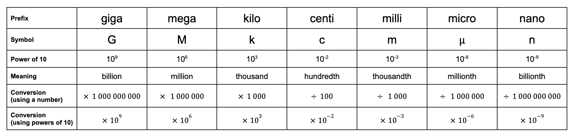
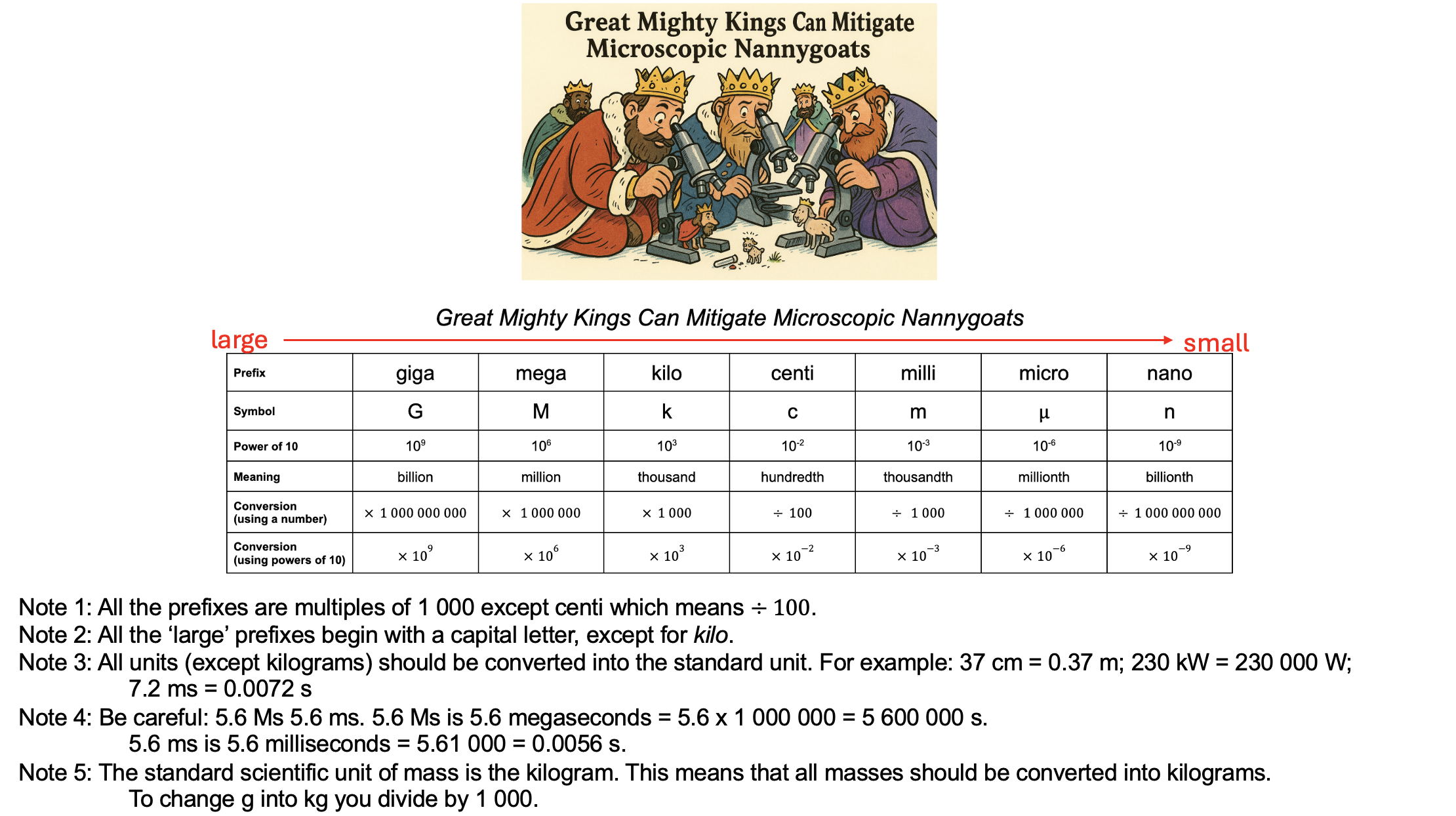
As of the time of writing, GCSE Science (2015 specification) students are expected to know the SI unit prefixes from giga- to nano-.
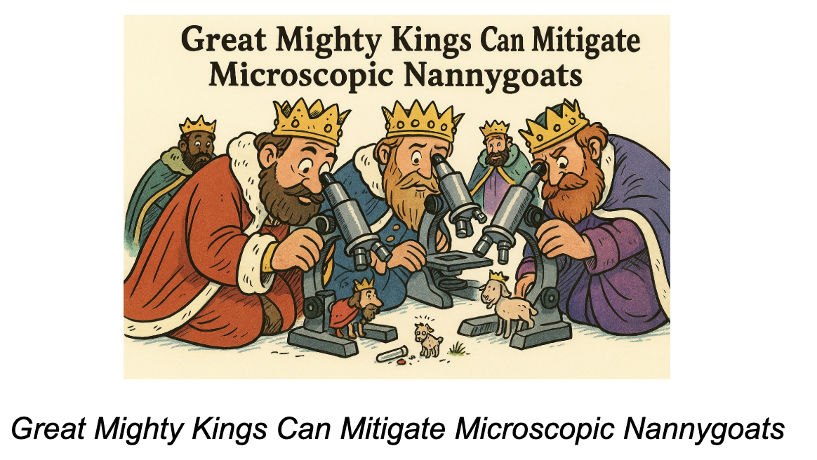
I suggest the following mnemonic:
A mnemonic for memorising the SI unit prefixes needed for GCSE
Choosing a mnemonic can be difficult because ‘mega’, ‘milli’ and ‘micro’ all begin with m, and even the first two letters of ‘milli’ and ‘micro’ are both ‘mi’. The mnemonic about helps students remember the difference between ‘milli’ and ‘micro’ by using ‘microscopic’ to help.
If you think this approach will be useful for your students, the Powerpoint is attached.
Enjoy!
PS You can find more of my thoughts on the SI system here
I recently made a bit of a mess of teaching the topic of gears by trying to ‘wing it’ with insufficient preparation. To avoid my — and possibly others’ — future blushes, I thought I would compile a post summarising my interpretation of what students need to know about gears for AQA GCSE Physics.
I am going to include some handy gifs and a clean, un-annotated Google Jamboard (my favoured medium for lessons).
Any continuing errors, omissions or misconceptions are entirely my own fault.
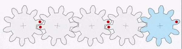
‘A simple gear system can be used to transmit the rotational effect of a force’ [AQA 4.5.4]
A gear is a wheel with teeth that can transmit the rotational effect of a force.
For example, in the gear train shown above, the first gear (A) is turned by a motor (green dot shown below). The moment (rotational effect) is passed via the interlocking teeth to gear B and so on down the chain to gear E. It is also worth pointing out that gear A has a clockwise moment but gear B has an anticlockwise moment. The direction alternates as we move down the chain. It takes a gear train of five gears to transmit the clockwise moment from gear A to gear E.
Gears A-E are all equal in size with the same number of teeth and, consequently, the moment does not change in magnitude as it passes down the chain (although, as noted above, it does change direction from clockwise to anticlockwise).
‘Students should be able to explain how gears transmit the rotational effect of forces’ [AQA 4.5.4]
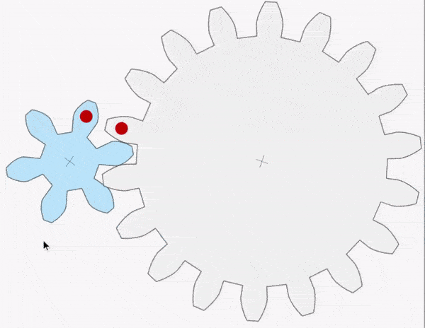
Part 1: A reduction gear arrangement
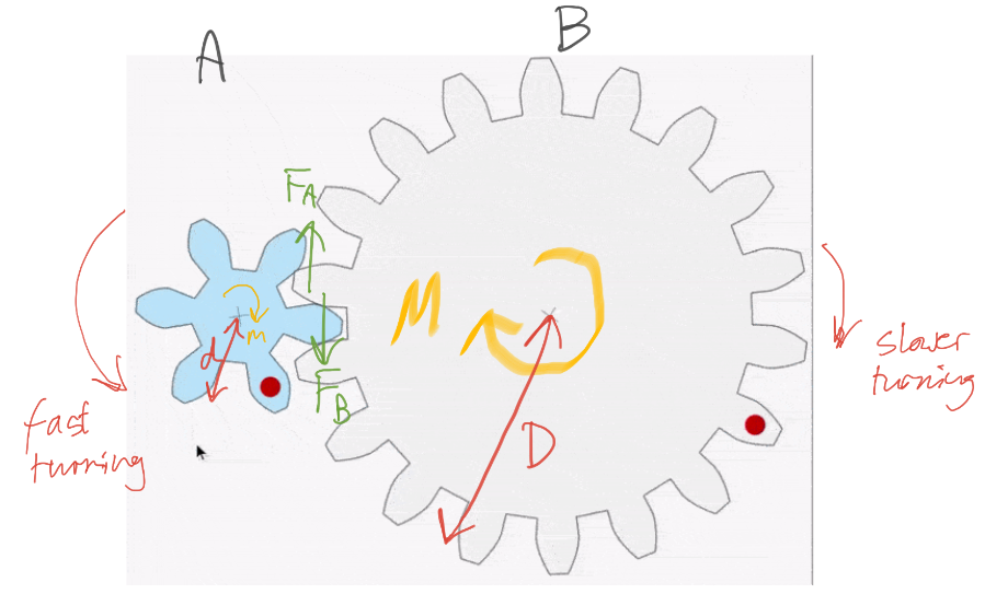
The driving gear (coloured blue) is smaller and has 6 teeth compared with the large gear’s 18 teeth. This is called a reduction gear arrangement.
A reduction gear arrangement does two things:
It slows down the speed of rotation. You may notice that the large gear turns only one for each three turns of the small gear.
The larger gear exerts a larger moment than the smaller gear. This is because the distance from the centre to the edge is larger for the grey gear.
The blue gear A exerts a force FA on gear B. By Newton’s Third Law, gear B exerts an equal but opposite force FB on gear A. Let’s take the magnitude of both forces to be F.
The anticlockwise moment exerted by gear A is given by m = F x d. The clockwise moment exerted by gear B is given by M=F x D. Since D > d then M > m.
A reduction gear arrangement is typically used in devices like an electric screwdriver. The electric motor in the device produces only a small rotational moment m but a large moment M is needed to turn the screws. The reduction gear produces the large moment M required.
Part 2: The overdrive arrangement
What happens when the driver gear is larger and has a greater number of teeth than the driven gear? This is called an overdrive arrangement.
The example we are going to look at is the arrangement of gears on a bicycle.
Here the driver gear (on the left) is linked via a chain to the smaller driven gear on the right. This means that the anticlockwise moment of the first gear is transmitted directly to the second gear as an anticlockwise moment. That is to say, the direction of the moment is not reversed as it is when the two gears are directly linked by interlocking teeth.
In the example shown, the big gear A turns only once for each four turns completed by the smaller gear B. Let’s assume that gear A exerts a force F on the chain so that the chain exerts an identical force F on gear B. Since D > d, this means that M > m so that the arrangement works as a distance multiplier rather than a force multiplier. This is, of course, excellent if we are riding at speed along a horizontal road. However, if we encounter an upward incline we may wish to — using the gear changing arrangement on the bike — swap the small gear B with one with a larger value of d. This would have the happy effect of increasing the magnitude of m so as to make it slightly easier to pedal uphill.
Rosencrantz (an anguished cry): CONSISTENCY IS ALL I ASK!
Tom Stoppard, Rosencrantz and Guildenstern Are Dead (1966)
I think that dual coding techniques can be extremely helpful in helping students understand the concept of change of momentum.
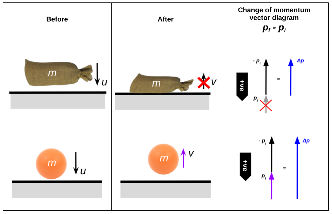
To engage our students’ physical intuitions, let’s consider a question like: Which would hurt more — being hit by a sandbag or being hit by a rubber ball?
Let’s assume that the sandbag and rubber ball have the same mass m and are travelling at the same initial velocity u. We choose ‘u‘ because it’s the initial velocity and we take ‘v‘ as the final velocity: a very subtle piece of dual coding that can reap rewards if applied consistently — pace Rosencrantz(!) — over a range of disparate examples.
We will use the change = final – initial convention (‘Consistency is all I ask!’)). The initial momentum is piand the final momentum is pf.
Now let’s work out the change in momentum in each case. We will assume that each item is dropped so that it impacts vertically on a horizontal surface. The velocity just before it hits is u so its initial momentum pi is given by pi = mu; its final velocity is v so its final momentum pf is given by pf = mv. The sandbag does not rebound, so its final velocity v is zero.
The rubber ball rebounds from the surface with a velocity v (we have shown that v < u so we are not assuming a perfectly elastic collision).
We will use the down-is-positive convention so that u is positive and the downward momentum pi are positive in both cases. However, the velocity v of the ball is negative so the momentum pf = mv is negative (upwards).
To add vectors, we simply put them ‘nose to tail’. However, in this case, we need to subtract the vectors, not add them. To do this, we use the operation pf + (-pi,). In other words, we put the vector pf nose to tail with minuspi, or with a vector pointing in the opposite direction to the original vector pi. These are shown in the table.
We can see that the change in momentum Δp is larger in the case of the rubber ball.
Applying Newton Second Law that force = change in momentum / change in time then (assuming the time of each interaction is the same) then we can conclude that the (upward) force exerted by the surface on the ball is larger than the force exerted by the surface on the sandbag.
From Newton’s Third Law (that if an object A exerts a force on object B, then object B exerts an equal and opposite force on object A), we can also conclude that the rubber exerts a larger downward force on the surface. This implies that, if the ball hit (say) your hand, then it would hurt more than the sandbag.
Considering change of momentum problems like this helps students answer questions such as the one shown below:
Exam question on change in momentum (solid black arrow and red arrow added)
We can discard options C and D since the change of momentum shown is in the wrong direction: the vertical component of momentum will remain unchanged.
A and B show changes of momentum of the same magnitude in the horizontal direction. However, if we take the horizontal component of the initial momentum as positive then the change of momentum on the gas particle must be negative; this implies that the correct answer is B.
Note also that diagram B shows the pf + (-pi) operation outlined above, with the arrow showing minus pi shown in red (added to the original exam question).
Do we delve deeply enough into the actual physical mechanism of current flow through electrical conductors (in terms of charge carriers and electric fields) in our treatments for GCSE and A-level Physics? I must reluctantly admit that I am increasingly of the opinion that the answer is no.
Of course, as physics teachers we talk with seeming confidence of current, potential difference and resistance but — when push comes to shove — can we (say) explain why a bulb lights up almost instantaneously when a switch several kilometres away is closed when the charge carriers can be shown to be move at a speed comparable to that of a sedate jogger? This would imply a time delay of some tens of minutes between closing the switch and energy being transferred from the power source (via the charge carriers) to the bulb.
When students asked me about this, I tended to suggest one of the following:
“The electrons in the wire are repelling each other so when one close to the power source moves, then they all move”; or
“Energy is being transferred to each charge carrier via the electric field from the power source.”
However, to be brutally honest, I think such explanations are too tentative and “hand wavy” to be satisfactory. And I also dislike being that well-meaning but unintentionally oh-so-condescending physics teacher who puts a stop to interesting discussions with a twinkly-eyed “Oh you’ll understand that when you study physics at degree level.” (Confession: yes, I have been that teacher too often for comfort. Mea culpa.)
Sherwood and Chabay (1999) argue that an approach to circuit analysis in terms of a predominately classical model of electrostatic charges interacting with electric fields is very helpful:
Students’ tendency to reason locally and sequentially about electric circuits is directly addressed in this new approach. One analyzes dynamically the behaviour of the *whole* circuit, and there is a concrete physical mechanism for how different parts of the circuit interact globally with each other, including the way in which a downstream resistor can affect conditions upstream.
(Side note: I think the Coulomb Train Model — although highly simplified and applicable only to a limited set of “steady state” situations — is consistent with Sherwood and Chabay’s approach, but more on that later.)
Misconception 1: “The electrons in a conductor push each other forwards.”
On this model, the flowing electrons push each other forwards like water molecules pushing neighbouring water molecules through a hose. Each negatively charged electron repels every other negatively charged electron so if one free electron within the conductor moves, then the neighbouring free electrons will also move. Hence, by a chain reaction of mutual repulsion, all the electrons within the conductor will move in lockstep more or less simultaneously.
The problem with this model is that it ignores the presence of the positively charged ions within the metallic conductor. A conveniently arranged chorus-line of isolated electrons would, perhaps, behave analogously to the neighbouring water molecules in a hose pipe. However, as Sherwood and Chabay argue:
Averaged over a few atomic diameters, the interior of the metal is everywhere neutral, and on average the repulsion between flowing electrons is canceled by attraction to positive atomic cores. This is one of the reasons why an analogy between electric current and the flow of water can be misleading.
The flowing electrons inside a wire cannot push each other through the wire, because on average the repulsion by any electron is canceled by the attraction of a nearby positive atomic core (Diagram from Sherwood and Chabay 1999: 4)
Misconception 2: “The charge carriers move because of the electric field from the battery.”
Let’s model the battery as a high-capacity parallel plate capacitor. This will avoid the complexities of having to consider chemical interactions within the cells. Think of a “quasi-steady state” where the current drawn from the capacitor is small so that electric charge on the plates remains approximately constant; alternatively, think of a mechanical charge transfer mechanism similar to the conveyor belt in a Van de Graaff generator which would be able to keep the charge on each plate constant and hence the potential difference across the plates constant (see Sherwood and Chabay 1999: 5).
A representation of the electric field around a single cell battery (modelled as a parallel plate capacitor)
This is not consistent with what we observe. For example, if the charge-carriers-move-due-to-electric-field-of the-battery model was correct then we would expect a bulb closer to the battery to be brighter than a more distant bulb; this would happen because the bulb closer to the battery would be subject to a stronger electric field and so we would expect a larger current.
A bulb closer to the battery is NOT brighter than a bulb further away from the battery (assuming negligible resistance in the connecting wires)
There is the additional argument if we orient the bulb so that the current flow is perpendicular to the electric field line, then there should be no current flow. Instead, we find that the orientation of the bulb relative to the electric field of the battery has zero effect on the brightness of the bulb.
There is no change of brightness as the orientation of the bulb is changed with respect to the electric field lines from the battery
Since we do not observe these effects, we can conclude that the electric field lines from the battery are not solely responsible for the current flow in the circuit.
Understanding the cause of current flow
If the electric field of the battery is not responsible on its own for the potential difference that causes a current to flow, where does the electric field come from?
Interviews reveal that students find the concept of voltage difficult or incomprehensible. It is not known how many students lose interest in physics because they fail to understand basic concepts. This number may be quite high. It is therefore astonishing that this unsatisfactory situation is accepted by most physics teachers and authors of textbooks since an alternative explanation has been known for well over one hundred years. The solution […] was in principle discovered over 150 years ago. In 1852 Wilhelm Weber pointed out that although a current-carrying conductor is overall neutral, it carries different densities of charges on its surface. Recognizing that a potential difference between two points along an electric circuit is related to a difference in surface charges [is the answer].
Härtel (2021): 21
We’ll look at these interesting ideas in part two.
[Note: this post edited 10/7/22 because of a rewritten part two]
I was “awoken from my dogmatic slumbers” on this topic (and alerted to Sherwood and Chabay’s treatment) by Youtuber Veritasium‘s provocative videos (see here and here).
Any sufficiently advanced technology is indistinguishable from magic.
Profiles of the Future (1962)
So wrote Arthur C. Clarke, science fiction author and the man who invented the geosynchronous communications satellite.
Clarke later joked of his regret at the billions of dollars he had lost by not patenting the idea, but one gets the impression that what really rankled him was another (and, to be fair, uncharacteristic) failure of imagination: he did not foresee how small and powerful solid state electronics would become. He had pictured swarms of astronauts crewing vast orbital structures, having their work cut out as they strove to maintain and replace the thousands of thermionic valves burning out under the weight of the radio traffic from Earth . . .
A communications nexus that could fit into a volume the size of a minibus, then (as the technology developed) a suitcase and then a pocket seemed implausible to him — and to pretty much everyone else as well.
And yet, here we are, living in the world that microelectronics has wrought. We are truly in an age of Clarkeian magic: our technology has become so powerful, so reliable and so ubiquitous — and so few of us have a full understanding of how it actually works — that it is very nearly indistinguishable from magic.
I want to outline a fictional vignette on the same theme which Clarke wrote in 1961 which has stayed with me since I read it. Please bear with me while I sketch out the story — it will lend some perspective to what follows.
In the novel A Fall of Moondust (1961) set in the year 2100, the lunar surface transport Selene has become trapped under fifteen metres of moondust. Rescue teams on the surface have managed to drill down to the stricken vessel with a metal pipe to supply the unfortunate passengers and crew with oxygen from the rescue ship. Communication would seem to be impossible as the Selene’s radio has been destroyed, but luckily Chief Engineer (Earthside) Lawrence has a plan:
They would hear his probe, but there was no way in which they could communicate with him. But of course there was. The easiest and most primitive means of all, which could be so readily overlooked after a century and a half of electronics.
A few hours later, the rescue team’s pipe drills through the roof of the sunken vessel.
The brief rush of air gave everyone a moment of unnecessary panic as the pressure equalised. Then the pipe was open to the upper world, and twenty two anxious men and women waited for the first breath of oxygen to come gushing down it.
Instead, the tube spoke.
Out of the open orifice came a voice, hollow and sepulchral, but perfectly clear. It was so loud, and so utterly unexpected, that a gasp of surprise came from the company. Probably not more than half a dozen of these men and women had ever heard of a ‘speaking tube’; they had grown up in the belief that only through electronics could the voice be sent across space. This antique revival was as much a novelty to them as a telephone would have been to an ancient Greek.
The humble converging lens as an ‘antique revival’
If you hold a magnifying glass (or any converging lens) in front of a white screen, then it will produce a real, inverted image of any bright objects in front of it. This simple act can, believe it or not, draw gasps of surprise from groups of our ‘digital native’ students: they assume that images can only be captured electronically. The fact that a shaped piece of glass can do so is as much a novelty to them as an LCD screen would have been to Galileo.
Think about it for a moment: how often has one of our students seen an image projected by a lens onto a passive screen? The answer is: possibly never.
The cinema? Not necessarily — many cinemas use large electronic screens now; there is no projection room, no projector painting the action on the screen from behind us with ghostly, dancing fingers of light. School? In the past, we had overhead projectors and even interactive whiteboards had lens systems, but these have largely been replaced by LED and LCD screens.
I believe that if you do not take the time to show the phenomenon of a single converging lens projecting a real image on to a passive white screen to your students, they are likely to have no familiar point of reference on which to build their understanding and lens diagrams will remain a puzzling set of lines that have little or no connection to their world.
Teaching Ray Diagrams
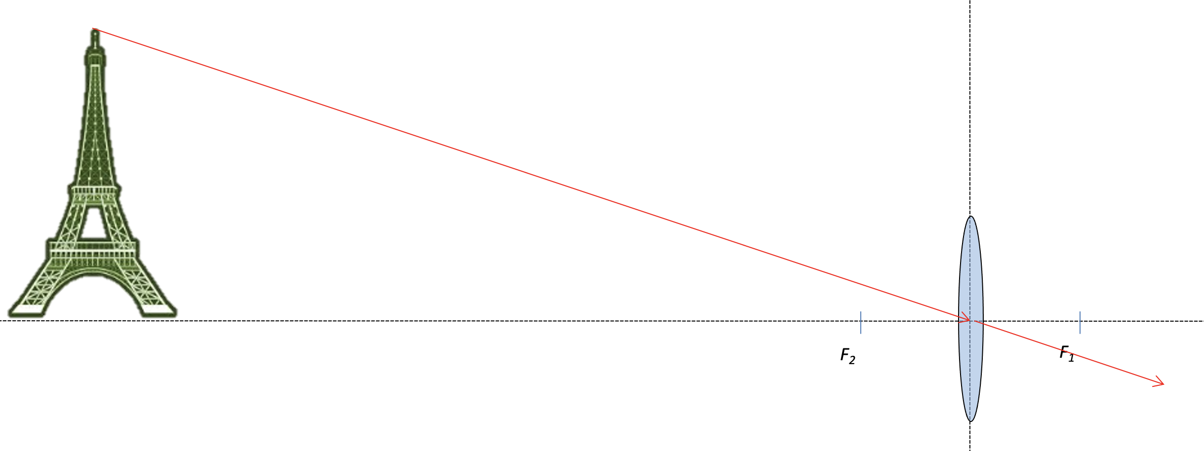
Start with a slide that looks something like this:
What represents the lens? The answer is not the blue oval. On ray diagrams, the lens is represented by the vertical dotted line. F1 and F2 are the focal points of this converging lens and they are each a distance f from the centre of the lens, where f is the focal length.
Now what happens to a light ray from the object that passes through the optical centre of the lens?
The answer, of course, is a big fat nothing. Light rays which pass through the optical centre of a thin lens are undeviated.
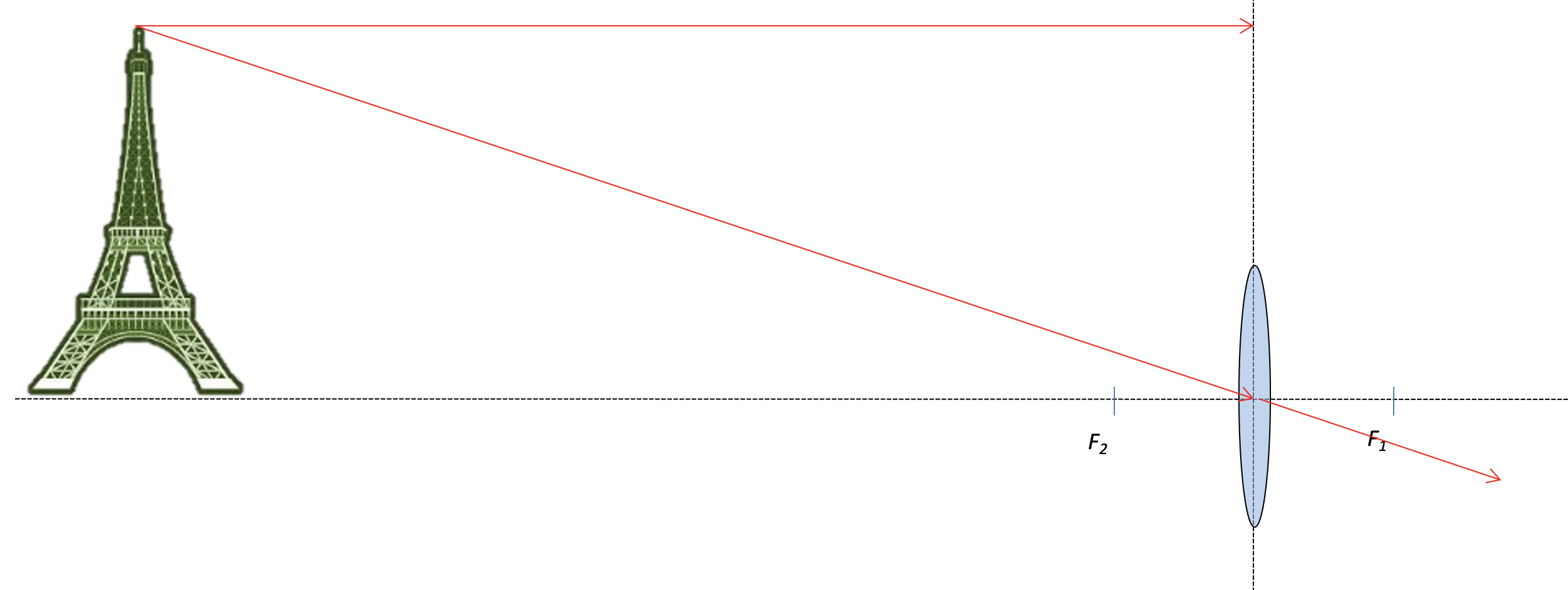
Now let’s track what happens to a light ray that travels parallel to the principal axis as shown?
Make sure that your students are aware that this light ray hasn’t ‘missed’ the lens. The lens is the vertical dotted line, not the blue oval. What will happen is that it will be deviated so that it passes through F1 (this is because this is a converging lens; if it had been a diverging lens then it would be be bent so that it appeared to come from F2).
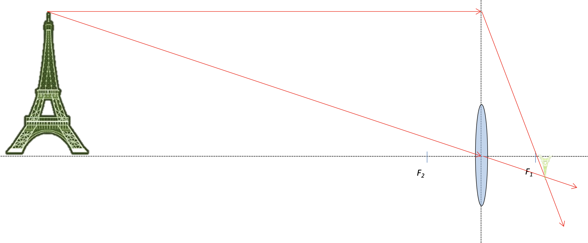
The image is formed where the two light rays cross, as shown below.
We can see that the image is inverted and reduced.
The image is formed close to F1 but not precisely at F1. This is because, although the object is distant from the lens (‘distant’ in this case being ‘further than 2f away’) it is not infinitely far away. However, the further we move the object away from the lens, then the closer to F1 the image is formed. The image will be formed a distance f from the screen when the object in very, very, very large distance away — or an ‘infinite distance’ away, if you prefer.
One of my physics teachers liked to say that ‘Infinity starts at the window sill’. In the context of thinking about lenses, I think he was right . . .
The PowerPoint that I used to produce the ray diagrams above is here. It is imperfect in a lot of ways but. truth be told, it has served me well over a number of years. It also features some other slides and animations that you may find useful — enjoy!
The phrase ‘Through a glass, darkly’ comes from the writings of the apostle Paul:
For now we see through a glass, darkly; but then face to face: now I know in part; but then shall I know even as also I am known.
KJV 1 Corinthians 13:12
The New International Version translates the phrase less poetically as ‘Now we see but a poor reflection as in a mirror.’
It has been argued that the ‘glass’ Paul was referring to were pieces of naturally-occurring semi-transparent mineral that were used in the ancient world as lenses or windows. They tended to produce a recognisable but distorted view of the world — hence, ‘darkly’.
Better technology means that there is much less distortion produced by our glasses — hence, ‘through a glass, lightly’.
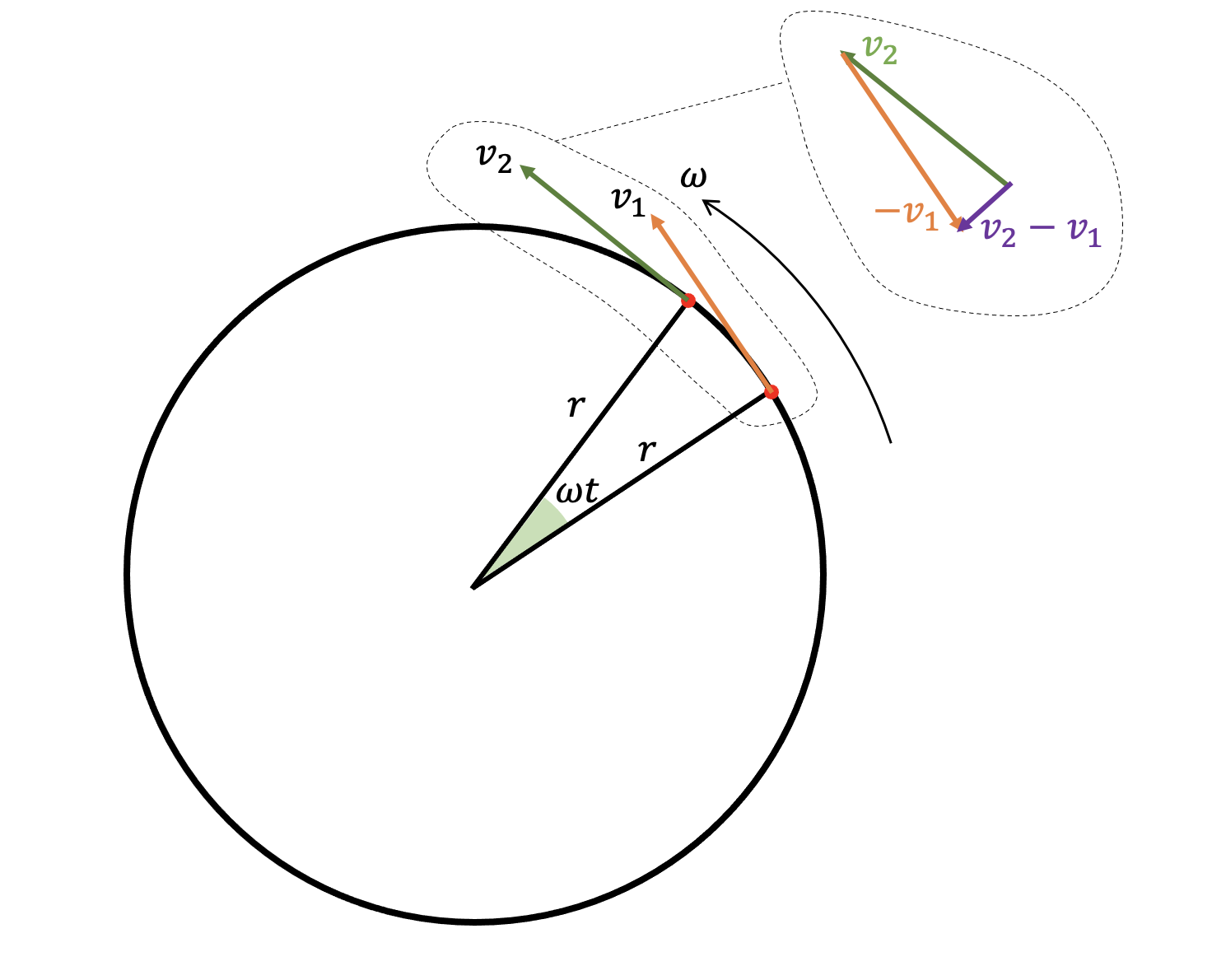
When I was an A-level physics student (many, many years ago, when the world was young LOL) I found the derivation of the centripetal acceleration formula really hard to understand. What follows is a method that I have developed over the years that seems to work well. The PowerPoint is included at the end.
Step 1: consider an object moving on a circular path
Let’s consider an object moving in circular path of radius r at a constant angular speed of ω (omega) radians per second.
The object is moving anticlockwise on the diagram and we show it at two instants which are time t seconds apart. This means that the object has moved an angular distance of ωt radians.
Step 2: consider the linear velocities of the object at these times
The linear velocity is the speed in metres per second and acts at a tangent to the circle, making a right angle with the radius of the circle. We have called the first velocity v1 and the second velocity at the later time v2.
Since the object is moving at a constant angular speed ω and is a fixed radius r from the centre of the circle, the magnitudes of both velocities will be constant and will be given by v = ωr.
Although the magnitude of the linear velocity has not changed, its direction most certainly has. Since acceleration is defined as the change in velocity divided by time, this means that the object has undergone acceleration since velocity is a vector quantity and a change in direction counts as a change, even without a change in magnitude.
Step 3a: Draw a vector diagram of the velocities
We have simply extracted v1 and v2 from the original diagram and placed them nose-to-tail. We have kept their magnitude and direction unchanged during this process.
Step 3b: close the vector diagram to find the resultant
The dark blue arrow is the result of adding v1 and v2. It is not a useful operation in this case because we are interested in the change in velocity not the sum of the velocities, so we will stop there and go back to the drawing board.
Step 3c switch the direction of velocity v1
Since we are interested in the change in velocity, let’s flip the direction of v1 so that it going in the opposite direction. Since it is opposite to v1, we can now call this -v1.
It is preferable to flip v1 rather than v2 since for a change in velocity we typically subtract the initial velocity from the final velocity; that is to say, change in velocity = v2 – v1.
Step 3d: Put the vectors v2 and (-v1) nose-to-tail
Step 3e: close the vector diagram to find the result of adding v2 and (-v1)
The purple arrow shows the result of adding v2 + (-v1); in other words, the purple arrow shows the change in velocity between v1 and v2 due to the change in direction (notwithstanding the fact that the magnitude of both velocities is unchanged).
It is also worth mentioning that that the direction of the purple (v2 –v1) arrow is in the opposite direction to the radius of the circle: in other words, the change in velocity is directed towards the centre of the circle.
Step 4: Find the angle between v2 and (-v1)
The angle between v2 and (-v1) will be ωt radians.
Step 5: Use the small angle approximation to represent v2-v1 as the arc of a circle
If we assume that ωt is a small angle, then the line representing v2-v1 can be replaced by the arc c of a circle of radius v (where v is the magnitude of the vectors v1 and v2 and v=ωr).
We can then use the familiar relationship that the angle θ (in radians) subtended at the centre of a circle θ = arc length / radius. This lets express the arc length c in terms of ω, t and r.
And finally, we can use the acceleration = change in velocity / time relationship to derive the formula for centripetal acceleration we a = ω2r.
Well, that’s how I would do it. If you would like to use this method or adapt it for your students, then the PowerPoint is attached.
Please Like or leave a comment if you find this useful 🙂
It is a thing plainly repugnant . . . to Minister the Sacraments in a Tongue not understanded of the People.
Gilbert, Bishop of Sarum. An exposition of the Thirty-nine articles of the Church of England (1700)
How can we help our students understand physics better? Or, in more poetic language, how can we make physics a thing that is more ‘understanded of the pupils’?
Redish and Kuo (2015: 573) suggest that the Resources Framework being developed by a number of physics education researchers can be immensely helpful.
In summary, the Resources Framework models a student’s reasoning as based on the activation of a subset of cognitive resources. These ‘thinking resources’ can be classified broadly as:
Embodied cognition: these are simple, irreducible cognitive resources sometimes referred to as ‘phenomenological primitives’ or p-prims such as ‘if-resistance-increases-then-the-output-decreases‘ and ‘two-opposing-effects-can-result-in-a-state-of-dynamic-balance‘. They are typically straightforward and ‘obvious’ generalisations of our lived, everyday experience as we move through the physical world. Embodied cognition is perhaps summarised as our ‘sense of mechanism’.
Encyclopedic (ancillary) knowledge: this is a complex cognitive resource made of a large number of highly interconnected elements: for example, the concept of ‘banana’ is linked dynamically with the concept of ‘fruit’, ‘yellow’, ‘curved’ and ‘banana-flavoured’ (Redish and Gupta 2009: 7). Encyclopedic knowledge can be thought of as the product of both informal and formal learning.
Contextualisation: meaning is constructed dynamically from contextual and other clues. For example, the phrase ‘the child is safe‘ cues the meaning of ‘safe‘ = ‘free from the risk of harm‘ whereas ‘the park is safe‘ cues an alternative meaning of ‘safe‘ = ‘unlikely to cause harm‘. However, a contextual clue such as the knowledge that a developer had wanted to but failed to purchase the park would make the statement ‘the park is safe‘ activate the ‘free from harm‘ meaning for ‘safe‘. Contextualisation is the process by which cognitive resources are selected and activated to engage with the issue.
Using the Resources Framework for teaching
I have previously used aspects of the Resources Framework in my teaching and have found it thought provoking and helpful to my practice. However, the ideas are novel and complex — at least to me — so I have been trying to think of a way of conveniently organising them.
What follows in my ‘first draft’ . . . comments and suggestions are welcome!
The RGB Model of the Resources Framework
The RGB Model of the Resources Framework
The red circle (the longest wavelength of visible light) represents Embodied Cognition: the foundation of all understanding. As Kuo and Redish (2015: 569) put it:
The idea is that (a) our close sensorimotor interactions with the external world strongly influence the structure and development of higher cognitive facilities, and (b) the cognitive routines involved in performing basic physical actions are involved in even in higher-order abstract reasoning.
The green circle (shorter wavelength than red, of course) represents the finer-grained and highly-interconnected Encyclopedic Knowledge cognitive structures.
At any given moment, only part of the [Encyclopedic Knowledge] network is active, depending on the present context and the history of that particular network
Redish and Kuo (2015: 571)
The blue circle (shortest wavelength) represents the subset of cognitive resources that are (or should be) activated for productive understanding of the context under consideration.
A human mind contains a vast amount of knowledge about many things but has limited ability to access that knowledge at any given time. As cognitive semanticists point out, context matters significantly in how stimuli are interpreted and this is as true in a physics class as in everyday life.
Redish and Kuo (2015: 577)
Suboptimal Understanding Zone 1
A common preconception held by students is that the summer months are warmer because the Earth is closer to the Sun during this time of year.
The combination of cognitive resources that lead students to this conclusion could be summarised as follows:
Encyclopedic knowledge: the Earth’s orbit is elliptical
Embodied cognition: The closer to a heat source you are the warmer it is.
Both of these cognitive resources, considered individually, are true. It is their inappropriate selection and combination that leads to the incorrect or ‘Suboptimal Understanding Zone 1’.
To address this, the RF(RGB) suggests a two pronged approach to refine the contextualisation process.
Firstly, we should address the incorrect selection of encyclopedic knowledge. The Earth’s orbit is elliptical but the changing Earth-Sun distance cannot explain the seasons because (1) the point of closest approach is around Jan 4th (perihelion) which is winter in the northern hemisphere; (2) seasons in the northern and southern hemispheres do not match; and (3) the Earth orbit is very nearly circular with an eccentricity e of 0.0167 where a perfect circle has e = 0.
Secondly, the closer-is-warmer p-prim is not the best embodied cognition resource to activate. Rather, we should seek to activate the spread-out-is-less-intense ‘sense of mechanism’ as far as we are able to (for example by using this suggestion from the IoP).
Suboptimal Understanding Zone 2
Another common preconception held by students is all waves have similar properties to the ‘breaking’ waves on a beach and this means that the water moves with the wave.
The structure of this preconception could be broken down into:
Embodied cognition: if I stand close to the water on a beach, then the waves move forward to wash over my feet.
Encyclopaedic knowledge: the waves observed on a beach are water waves
Considered in isolation, both of these cognitive resources are unproblematic: they accurately describes our everyday, lived experience. It is the contextualisation process that leads us to apply the resources inappropriately and places us squarely in Suboptimal Understanding Zone 2.
The RF(RGB) Model suggests that we can address this issue in two ways.
Firstly, we could seek to activate a more useful embodied cognition resource by re-contextualising. For example, we could ask students to imagine themselves floating in deep water far from the shore: do the waves carry them in any particular direction or simply move them up or down as they pass by?
Secondly, we could seek to augment their encyclopaedic knowledge: yes, the waves on a beach are water waves but they are not typical water waves. The slope of the beach slows down the bottom part of the wave so the top part moves faster and ‘topples over’ — in other words, the water waves ‘break’ leading to what appears to be a rhythmic back-and-forth flow of the waves rather than a wave train of crests and troughs arriving a constant wave speed. (This analysis is over a short period of time where the effect of any tidal effects is negligible.)
Both processes try to ‘tug’ student understanding into the central, optimal zone.
Suboptimal Understanding Zone 3
Redish and Kuo (2015: 585) recount trying to help a student understand the varying brightness of bulbs in the circuit shown.
All bulbs are identical. Bulbs A and D are bright; bulbs B and C are dim.
The student said that they had spent nearly an hour trying to set up and solve the Kirchoff’s Law loop equations to address this problem but had been unsuccessful in accounting for the varying brightnesses.
Redish suggested to the student that they try an analysis ‘without the equations’ and just look at the problems in simpler physical terms using just the concept of electric current. Since current is conserved it must split up to pass through bulbs B and C. Since the brightness is dependent on the current, the smaller currents in B and C compared with A and D accounts for their reduced brightness.
When he was introduced to [this] approach to using the basic principles, he lit up and was able to solve the problem quickly and easily, saying, ‘‘Why weren’t we shown this way to do it?’’ He would still need to bring his conceptual understanding into line with the mathematical reasoning needed to set up more complex problems, but the conceptual base made sense to him as a starting point in a way that the algorithmic math did not.
Analysing this issue using the RF(RGB) it is plausible to suppose that the student was trapped in Suboptimal Understanding Zone 3. They had correctly selected the Kirchoff’s Law resources from their encyclopedic knowledge base, but lacked a ‘sense of mechanism’ to correctly apply them.
What Redish did was suggest using an embodied cognition resource (the idea of a ‘material flow’) to analyse the problem more productively. As Redish notes, this wouldn’t necessarily be helpful for more advanced and complex problems, but is probably pedagogically indispensable for developing a secure understanding of Kirchoff’s Laws in the first place.
Conclusion
The RGB Model is not a necessary part of the Resources Framework and is simply my own contrivance for applying the RF in the context of physics education at the high school level. However, I do think the RF(RGB) has the potential to be useful for both physics and science teachers.
Hopefully, it will help us to make all of our subject content more ‘understanded of the pupils’.
References
Redish, E. F., & Gupta, A. (2009). Making meaning with math in physics: A semantic analysis. GIREP-EPEC & PHEC 2009, 244.
Redish, E. F., & Kuo, E. (2015). Language of physics, language of math: Disciplinary culture and dynamic epistemology. Science & Education, 24(5), 561-590.
A huge thank you to everyone who has viewed, read or commented on one of my posts in 2021: whether you agreed or disagreed with my point of view, you are the people that make the work of writing this blog so enjoyable and rewarding.
The top 3 most-read posts of 2021 were:
1. What to do if your school has a batshit crazy marking policy
This particular post was written back in 2019 and it’s sobering to realise that it is still relevant enough that it was featured by @TeacherTapp in November 2021. As edu-blog writers will know, this unlooked for honour generates thousands of views — thanks, @TeacherTapp!
Note to schools: please, if you haven’t done so already, please please please sort out your marking policy and make sure it is workable and fit for purpose. It would seem that, even now, teachers are being made to mark for the sake of marking, rather than for any tangible educational benefit.
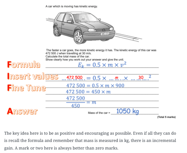
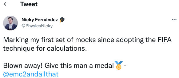
2. FIFA for the GCSE Physics Calculation Win!
The next post is one I am very proud of, even though FIFA is just a silly mnemonic to help students follow the “substitute-first-and-then-rearrange” method favoured by AQA mark schemes. Yes, FIFA did start life as a “mark-grubbing” dodge; however, somewhat to my own surprise, I found that the vast majority of students (LPAs included), can rearrange successfully if they substitute the numbers in first. Many other teachers have found the same thing as well — search #FIFAcalc on Twitter for some illustrative tweets from FIFAcalc’s biggest fans.
However, it is clear that the formula triangle method still has many adherents. I think this is unfortunate because: (a) they only work for a limited subset of formulas with the format y=mx; (b) they are a cognitive dead end that actively block students from accessing higher level STEM courses; and (c) as Ed Southall argues effectively, they are a form of procedural teaching rather than conceptual teaching.
3. Why does kinetic energy = 1/2mv^2?
This post is a surprise “sleeper” hit also dating from 2019. It outlines an accessible method for deriving the kinetic energy formula. From getting a respectable but niche 200 views per year in 2019 and 2020, in 2021 it shot up to over 3K views. What is very encouraging for me is that most of these views come from internet searches by individuals from a wide range of backgrounds and not just my fellow denizens of the online edu-Bubble!
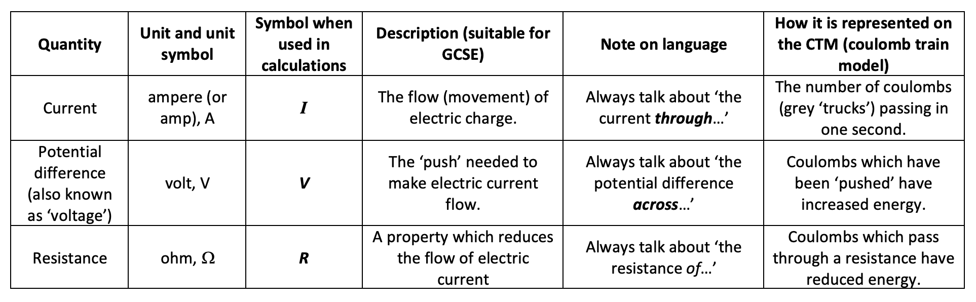
In this post, we will look at understanding potential difference (or voltage) using the Coulomb Train Model.
This is part 2 of a continuing series. You can read part 1 here.
The Coulomb Train Model (CTM) is a helpful model for both explaining and predicting the behaviour of real electric circuits which I think is suitable for use with KS3 and KS4 students (that’s 11-16 year olds for non-UK educators).
To summarise what has been discussed so far:
Modelling potential difference using the CTM
Potential difference is the ‘push’ needed to make electric charge move around a closed circuit. On the CTM, we can represent the ‘push’ as a gain in the energy of the coulomb. (This is consistent with the actual definition of the volt V = E/Q, where one volt is a change in energy of one joule per coulomb.)
How can we observe this gain in energy? Simple, we use a voltmeter.
What the voltmeter does is compare the energy contained by two coulombs: one at A and the other at B. The coulombs at B, having passed through the 1.5 V cell, each have 1.5 joules of energy more than than the coulombs at A. This means that the voltmeter in this position reads 1.5 volts. We would say that the potential difference across the cell is 1.5 V. (Try and avoid talking about the potential difference ‘through’ or ‘of’ any part of the circuit.)
More potential difference measurements using the CTM
Let’s move the voltmeter to a different position.
On the CTM, this would look like this:
Let’s make the very reasonable assumption that the connecting wires have zero resistance. This would mean that the coulombs at C have 1.5 joules of energy and that the coulombs at D have 1.5 joules of energy. They have not lost any energy since they have not passed through any part of the circuit that actually has a resistance. The voltmeter would therefore read 0 volts since it cannot detect any energy difference.
Now let’s move the voltmeter one last time.
On the CTM, this would look like this:
Notice that the coulombs at F have 1.5 fewer joules than the coulombs at E. The coulombs transfer 1.5 joules of energy to the bulb because the bulb has a resistance.
Any part of the circuit that has non-zero resistance will ‘rob’ coulombs of their energy. On this very simple model, we assume that only the bulb has a resistance and so only the bulb will ‘push back’ against the movement of the coulombs and cost them energy.
Also on this simple model, the potential difference across the bulb is identical to the potential difference across the cell — but this is not always the case. For example, if the wires had a small but non-negligible resistance and if the cell had an internal resistance, but these would only come into play at A-level.
The bulb is shown as ‘flashing’ on the CTM to provide a visual cue to help students mentally model the transfer of energy from the coulombs to the bulb. In reality, instead of just one coulomb transferring a largish ‘chunk’ of energy, there would be approximately 1.25 billion billion electrons continuously transferring a tiny fraction of this energy over the course of one second (assuming a d.c. current of 0.2 amps) so we wouldn’t see the bulb ‘flash’ in reality.
How do the coulombs ‘know’ how much energy to drop off?
This section is probably more of interest to specialist physics teachers, but all are welcome.
One frequent criticism of donation models like the CTM is how do the coulombs ‘know’ to drop off all their energy at the bulb?
The response to this, of course, is that they don’t. This criticism is an artefact of an (arguably) over-simplified model whereby we assume that only the bulb has resistance. The energy carried by the coulombs according to this model could be shown as a sketch graph, and let’s be honest it does look a little dodgy…
But, more accurately, of course, the energy loss is a process rather than an event. And the connecting wires actually have a small resistance. This leads to this graph:
Realistically speaking, the coulombs don’t lose all their energy passing through the bulb: they merely lose most of their energy here due to the process of passing through a high resistance part of the circuit.
In part 3 of this series, we’ll look at how resistance can be modelled using the CTM.
Batman gives a Physics-Six-Marker the ol’ FIFA-One-Two,
Many students struggle with Physics calculation questions at KS3 and KS4. Since 40% of the marks on GCSE Physics papers are for maths, this is a real worry for their teachers.
The FIFA system (if that’s not too grandiose a description) provides a minimal and flexible framework that helps students to successfully attempt calculation questions.
Since adopting the system, we encounter far fewer blanks on test and exam scripts where students simply skip over a calculation question. A typical student can gain 10-20 marks.
The FIFA system is outlined here but essentially consists of:
Formula: students write the formula or equation
Insert values: students insert the known data from the question.
Fine-tune: rearrange, convert units, simplify etc.
Answer: students state the final answer.
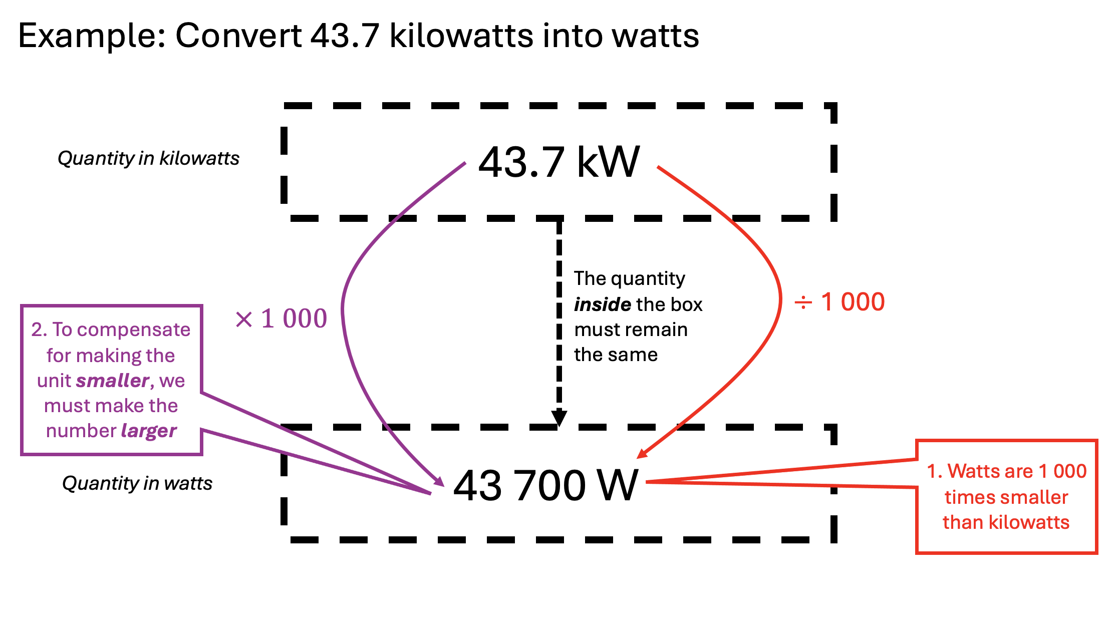
The “Fine-tune” stage is not — repeat, not — synonymous with re-arranging and is designed to be “creatively ambiguous” and allow space to “do what needs to be done” and can include unit conversion (e.g. kilowatts to watts), algebraic rearrangement and simplification.
The FIFA-One-Two
Uniquely for Physics, instead of the dreaded “Six Marker” extended writing question, we have the even-more-dreaded “Six Marker” long calculation question. (Actually, they can be awarded anywhere between 4 to 6 marks, but we’ll keep calling them “Six Markers” for convenience.)
The “FIFA-one-two” strategy can help students gain marks in these questions.
Let’s look how it could be applied to a typical “Six mark” long calculation question. We prepare the ground like this:
FIFA-one-two: the set up. (Note that since the expected unit of the final answer is given, this is actually a five marker not a six marker; however, the system works equally well in both cases.)
Since the question mentions the power output of the kettle first, let’s begin by writing down the energy transferred equation.
Next we insert the values. It’s quite helpful to write in any “non standard” units such as kilowatts, minutes etc as a reminder that these need to be converted in the Fine-tune phase.
And so we arrive at the final answer for this first section:
Next we write down the specific heat capacity equation:
And going through the second FIFA operation:
Conclusion
I think every “Six Marker” extended calculation question can be approached in a productive way using the FIFA-One-Two approach.
This means that, even if students can’t reach the final answer, they will pick up some method marks along the way.
I hope you give the FIFA-One-Two method a go with your students.