Circuit Diagrams: Lost in Rotation…?

Is there a better way of presenting circuit diagrams to our students that will aid their understanding of potential difference?

I think that, possibly, there may be.

(Note: circuit diagrams produced using the excellent — and free! — web editor at https://www.circuit-diagram.org/.)

Old ways are the best ways…? (Spoiler: not always)

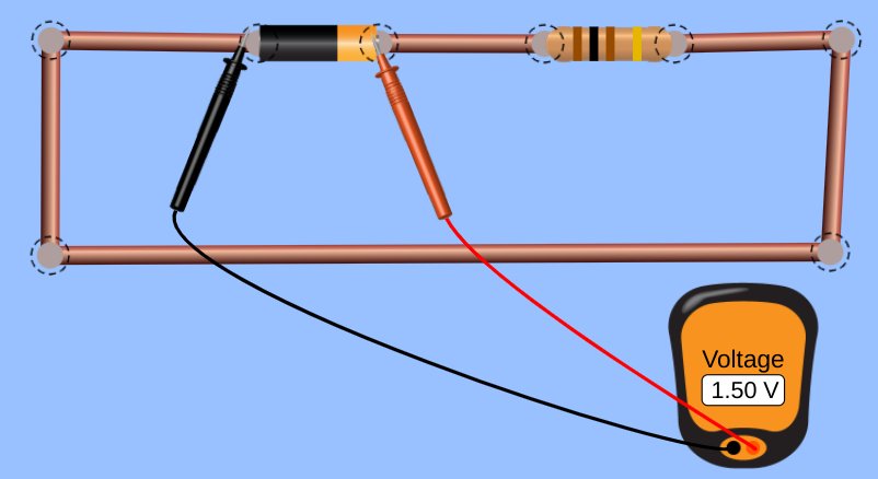
This is a very typical, conventional way of showing a simple circuit.

A simple circuit as usually presented

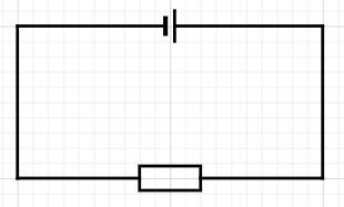
Now let’s measure the potential difference across the cell…

Measuring the potential difference across the cell

…and across the resistor.

Measuring the potential difference across the resistor

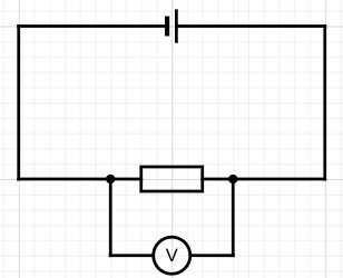
Using a standard school laboratory digital voltmeter and assuming a cell of emf 1.5 V and negligible internal resistance we would get a value of +1.5 volts for both positions.

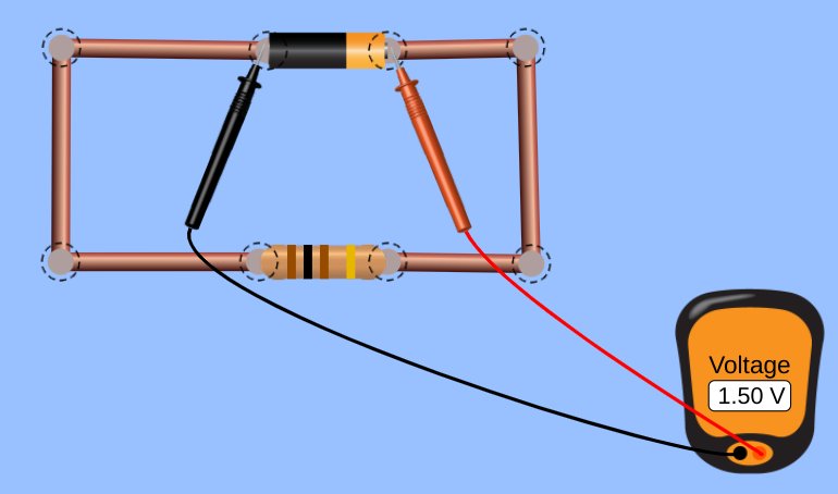
Let me demonstrate this using the excellent — and free! — pHET circuit simulation website.

Indeed, one might argue with some very sound justification that both measurements are actually of the same potential difference and that there is no real difference between what we chose to call ‘the potential difference across the cell’ and ‘the potential difference across the resistor’.
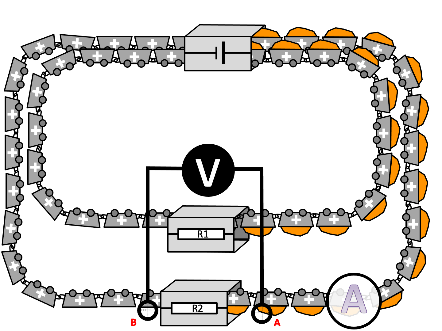
Try another way…

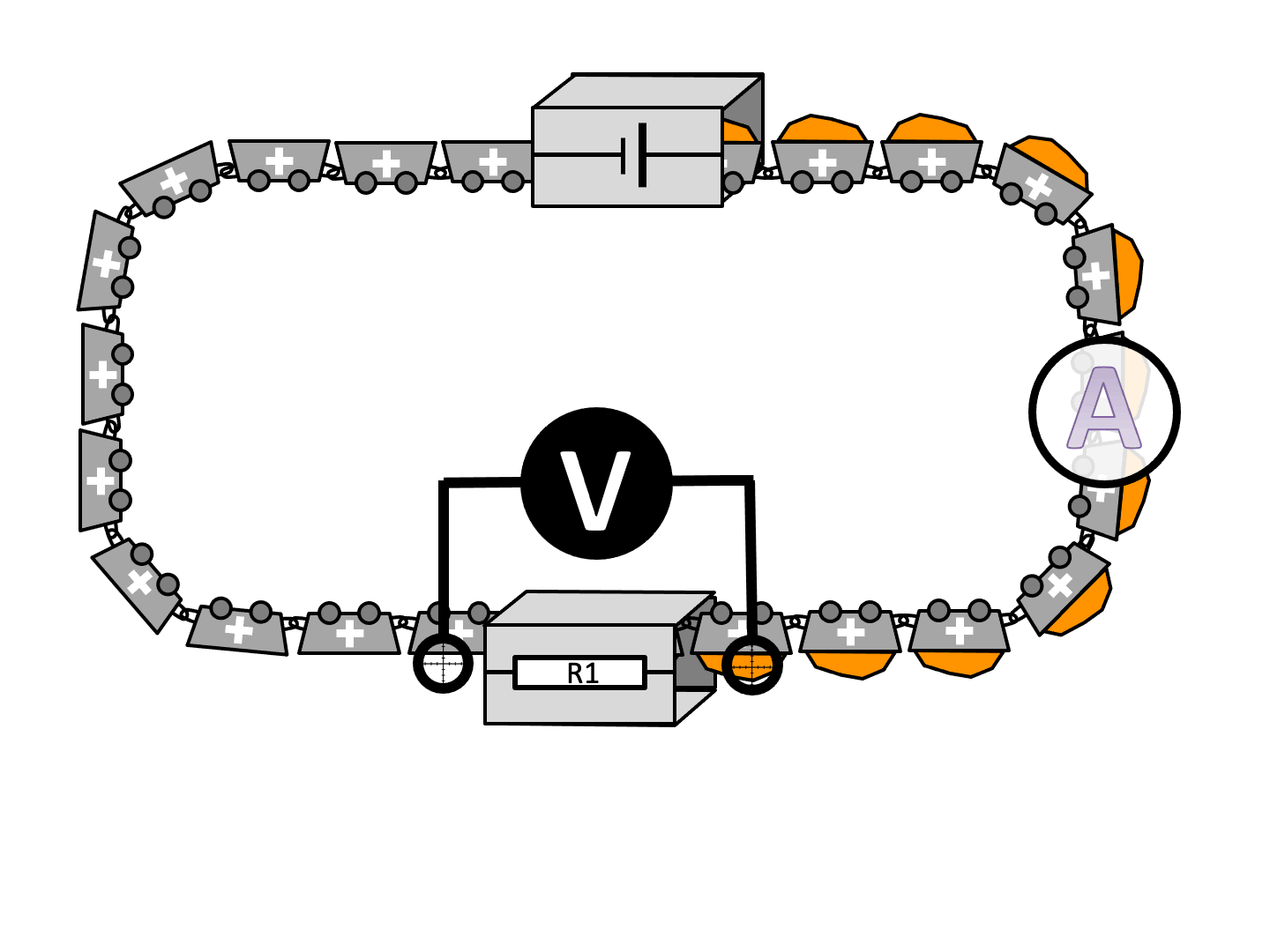
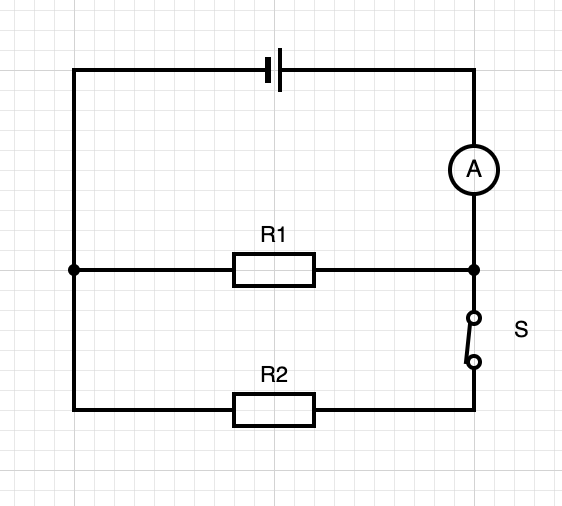
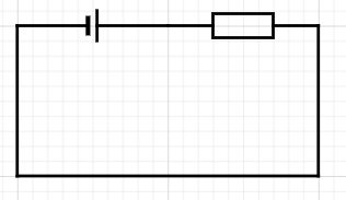
But let’s consider drawing the circuit a different (but operationally identical) way:

The same circuit drawn ‘all-in-a-row’

What would happen if we measured the potential difference across the cell and the resistor as before…

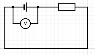
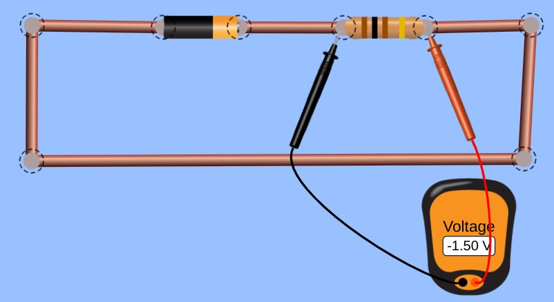
This time, we get a reading (same assumptions as before) of [positive] +1.5 volts of potential difference for the potential difference across the cell and [negative] -1.5 volts for the potential difference across the resistor.

This, at least to me, is a far more conceptually helpful result for student understanding. It implies that the charge carriers are gaining energy as they pass through the cell, but losing energy as they pass through the resistor.

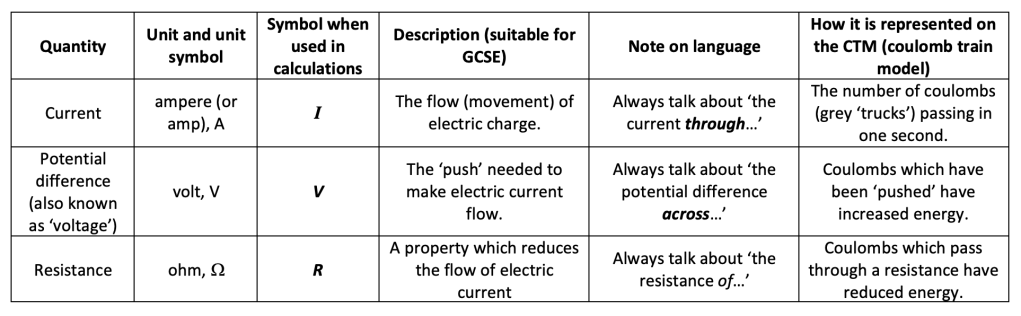
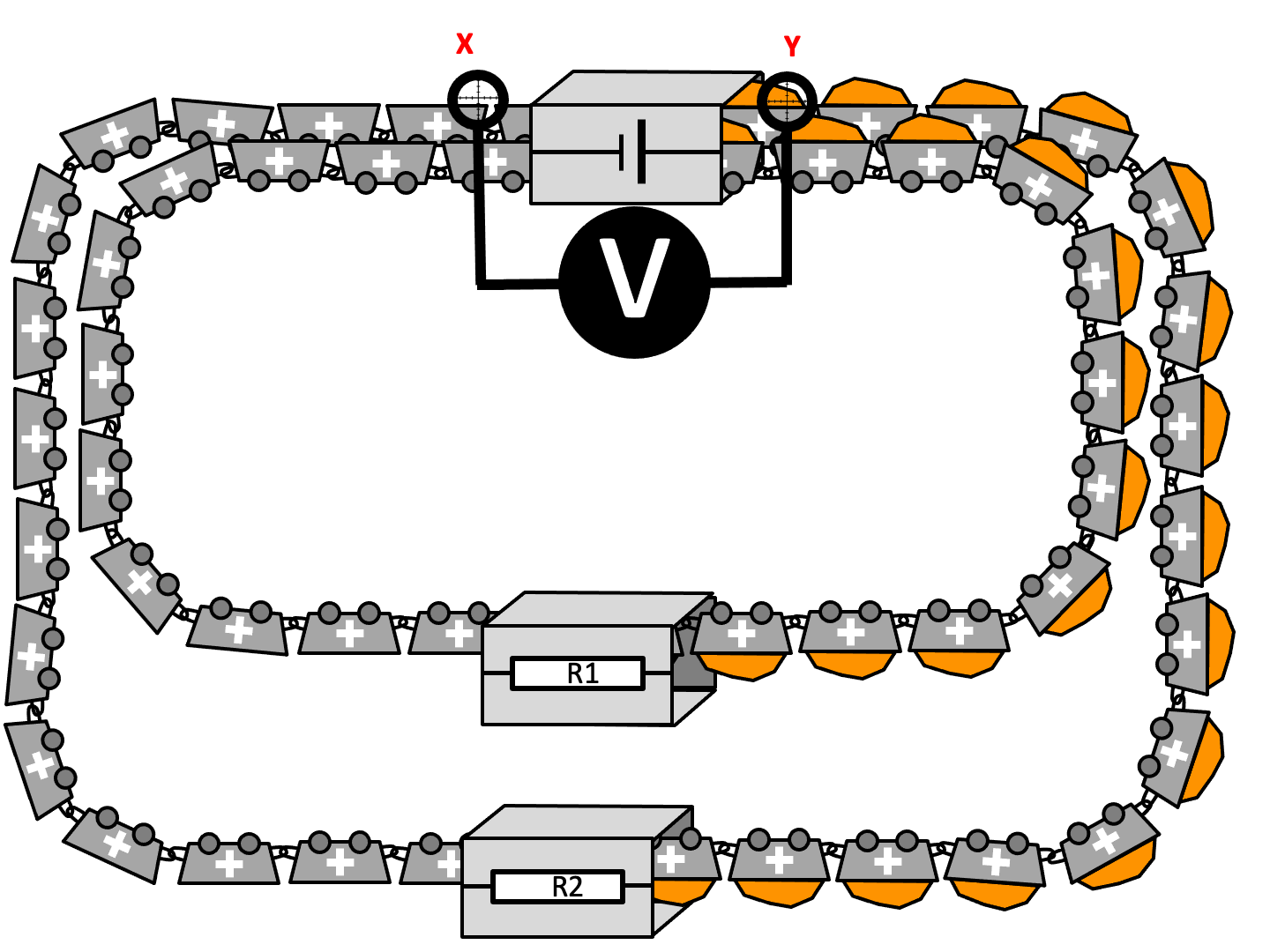
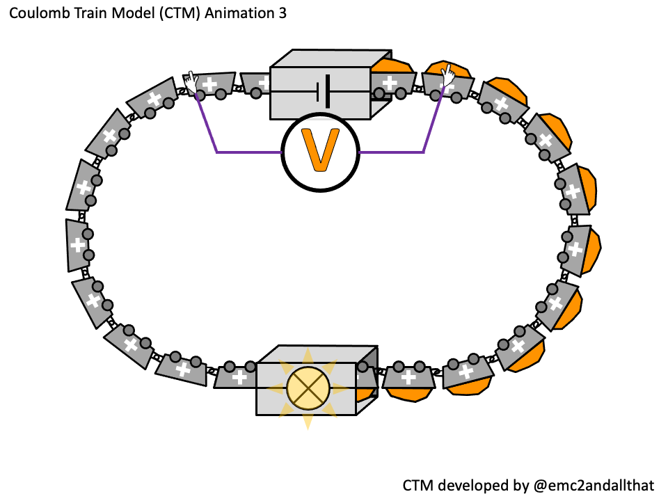
Using the Coulomb Train Model of circuit behaviour, this could be shown like this:

+1.5 V of potential difference represented using the Coulomb Train Model
-1.5 V of potential difference represented using the Coulomb Train Model. (Note: for a single resistor circuit, the emerging coulomb would have zero energy.)

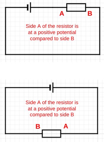
We can, of course, obtain a similar result for the conventional layout, but only at the cost of ‘crossing the leads’ — a sin as heinous as ‘crossing the beams’ for some students (assuming they have seen the original Ghostbusters movie).

Crossing the leads on a voltmeter

A Hidden Rotation?

The argument I am making is that the conventional way of drawing simple circuits involves an implicit and hidden rotation of 180 degrees in terms of which end of the resistor is at a more positive potential.

A hidden rotation…?

Of course, experienced physics learners and instructors take this ‘hidden rotation’ in their stride. It is an example of the ‘curse of knowledge’: because we feel that it is not confusing we fail to anticipate that novice learners could find it confusing. Wherever possible, we should seek to make whatever is implicit as explicit as we can.

Conclusion

A translation is, of course, a sliding transformation, rather than a circumrotation. Hence, I had to dispense with this post’s original title of ‘Circuit Diagrams: Lost in Translation’.

However, I do genuinely feel that some students understanding of circuits could be inadvertently ‘lost in rotation’ as argued above.

I hope my fellow physics teachers try introducing potential difference using the ‘all-in-row’ orientation shown.

The all-in-a-row orientation for circuit diagrams to help student understanding of potential difference

I would be fascinated to know if they feel its a helpful contribition to their teaching repetoire!

The Coulomb Train Model Revisited (Part 4)

In this post, we will look at parallel circuits.

The Coulomb Train Model (CTM) is a helpful model for both explaining and predicting the behaviour of real electric circuits which I think is useful for KS3 and KS4 students.

Without further ado, here is a a summary.

This is part 4 of a continuing series. (Click to read Part 1, Part 2 or Part 3.)


The ‘Parallel First’ Heresy

I advocate teaching parallel circuits before teaching series circuits. This, I must confess, sometimes makes me feel like Captain Rum from Blackadder Two:

The main reason for this is that parallel circuits are conceptually easier to analyse than series circuits because you can do so using a relatively naive notion of ‘flow’ and gives students an opportunity to explore and apply the recently-introduced concept of ‘flow of charge’ in a straightforward context.

Redish and Kuo (2015: 584) argue that ‘flow’ is an example of embodied cognition in the sense that its meaning is grounded in physical experience:

The thesis of embodied cognition states that ultimately our conceptual system grounded in our interaction with the physical world: How we construe even highly abstract meaning is constrained by and is often derived from our very concrete experiences in the physical world.

Redish and Kuo (2015: 569)

As an aside, I would mention that Redish and Kuo (2015) is an enduringly fascinating paper with a wealth of insights for any teacher of physics and I would strongly recommend that everyone reads it (see link in the Reference section).


Let’s Go Parallel First — but not yet

Let’s start with a very simple circuit.

This is not a parallel circuit (yet) because switch S is open. Resistors R1 and R2 are identical.

This can be represented on the coulomb train model like this:

Five coulombs pass through the ammeter in 20 seconds so the current I = Q/t = 5/20 = 0.25 amperes.

Let’s assume we have a 1.5 V cell so 1.5 joules of energy are added to each coulomb as they pass through the cell. Let’s also assume that we have negligible resistance in the cell and the connecting wires so 1.5 joules of energy will be removed from each coulomb as they pass through the resistor. The voltmeter as shown will read 1.5 volts.

The resistance of the resistor R1 is R=V/I = 1.5/0.25 = 6.0 ohms.


Let’s Go Parallel First — for real this time.

Now let’s close switch S.

This is example of changing an example by continuous conversion which removes the need for multiple ammeters in the circuit. The changed circuit can be represented on the CTM as shown

Now, ten coulombs pass through the ammeter in twenty seconds so I = Q/t = 10/20 = 0.5 amperes (double the reading in the first circuit shown).

Questioning may be useful at this point to reinforce the ‘flow’ paradigm that we hope students will be using:

  • What will be the reading if the ammeter moved to a similar position on the other side? (0.5 amps since current is not ‘used up’.)
  • What would be the reading if the ammeter was placed just before resistor R1? (0.25 amps since only half the current goes through R1.)

To calculate the total resistance of the whole circuit we use R = V/I = 1.5/0.5 = 3.0 ohms– which is half of the value of the circuit with just R1. Adding resistors in parallel has the surprising result of reducing the total resistance of the circuit.

This is a concrete example which helps students understand the concept of resistance as a property which reduces current: the current is larger when a second resistor is added so the total resistance must be smaller. Students often struggle with the idea of inverse relationships (i.e. as x increases y decreases and vice versa) so this is a point well worth emphasising.


Potential Difference and Parallel Circuits (1)

Let’s expand on the primitive ‘flow’ model we have been using until now and adapt the circuit a little bit.

This can be represented on the CTM like this:

Each coulomb passing through R2 loses 1.5 joules of energy so the voltmeter would read 1.5 volts.

One other point worth making is that the resistance of R2 (and R1) individually is still R = V/I = 1.5/0.25 = 6.0 ohms: it is only the combined effect of R1 and R2 together in parallel that reduces the total resistance of the circuit.


Potential Difference and Parallel Circuits (2)

Let’s have one last look at a different aspect of this circuit.

This can be represented on the CTM like this:

Each coulomb passing through the cell from X to Y gains 1.5 joules of energy, so the voltmeter would read 1.5 volts.

However, since we have twice the number of coulombs passing through the cell as when switch S is open, then the cell has to load twice as many coulombs with 1.5 joules in the same time.

This means that, although the potential difference is still 1.5 volts, the cell is working twice as hard.

The result of this is that the cell’s chemical energy store will be depleted more quickly when switch S is closed: parallel circuits will make cells go ‘flat’ in a much shorter time compared with a similar series circuit.

Bulbs in parallel may shine brighter (at least in terms of total brightness rather than individual brightness) but they won’t burn for as long.

To some ways of thinking, a parallel circuit with two bulbs is very much like burning a candle at both ends…


More fun and high jinks with coulomb train model in the next instalment when we will look at series circuits.

You can read part 5 here.


Reference

Redish, E. F., & Kuo, E. (2015). Language of physics, language of math: Disciplinary culture and dynamic epistemologyScience & Education24(5), 561-590.

The Coulomb Train Model Revisited (Part 1)

The Coulomb Train Model (CTM) is a helpful model for both explaining and predicting the behaviour of real electric circuits which I think is suitable for use with KS3 and KS4 students (that’s 11-16 year olds for non-UK educators).

I have written about it before (see here and here) but I have recently been experimenting with animated versions of the original diagrams.

Essentially, the CTM is a donation model akin to the famous ‘bread and bakery van’ or even the ‘penguins and ski lift’ models, but to my mind it has some major advantages over these:

  • The trucks (‘coulombs’) in the CTM are linked in a continuous chain. If one ‘coulomb’ stops then they all stop. This helps students grasp why a break anywhere in a circuit will stop all current.
  • The CTM presents a simplified but still quantitatively accurate picture of otherwise abstract entities such as coulombs and energy rather than the more whimsical ‘bread van’ = ‘charge carrier’ and ‘bread’ = ‘energy’ (or ‘penguin’ = ‘charge carrier’ and ‘gpe of penguin’ = ‘energy of charge carrier’) for the other models.
  • Explanations and predictions scripted using the CTM use direct but substantially correct terminiology such as ‘One ampere is one coulomb per second’ rather than the woolier ‘current is proportional to the number of bread vans passing in one second’ or similar.

Modelling current flow using the CTM

The coulombs are the ‘trucks’ travelling clockwise in this animation. This models conventional current.

Charge flow (in coulombs) = current (in amps) x time (in seconds)

So a current of one ampere is one coulomb passing in one second. On the animation, 5 coulombs pass through the ammeter in 25 seconds so this is a current of 0.20 amps.

We have shown two ammeters to emphasise that current is conserved. That is to say, the coulombs are not ‘used up’ as they pass through the bulb.

The ammeters are shown as semi-transparent as a reminder that an ammeter is a ‘low resistance’ instrument.


Modelling ‘a source of potential difference is needed to make current flow’ using the CTM

Energy transferred (in joules) = potential difference (in volts) x charge flow (in coulombs) 

So the potential difference = energy transferred divided by the number of coulombs.

The source of potential difference is the number of joules transferred into each coulomb as it passes through the cell. If it was a 1.5 V cell then 1.5 joules of energy would be transferred into each coulomb.

This is represented as the orange stuff in the coulombs on the animation.

What is this energy? Well, it’s not ‘electrical energy’ for certain as that is not included on the IoP Energy Stores and Pathways model. In a metallic conductor, it would be the sum of the kinetic energy stores and electrical potential energy stores of 6.25 billion billion electrons that make up one coulomb of charge. The sum would be a constant value (assuming zero resistance) but it would be interchanged randomly between the kinetic and potential energy stores.

For the CTM, we can be a good deal less specific: it’s just ‘energy’ and the CTM provides a simplified, concrete picture that allows us to apply the potential difference equation in a way that is consistent with reality.

Or at least, that would be my argument.

The voltmeter is shown connected in parallel and the ‘gloves’ hint at it being a ‘high resistance’ instrument.

More will follow in part 2 (including why I decided to have the bulb flash between bright and dim in the animations).

You can read part 2 here.