e=mc2andallthat

Gustav Robert Kirchhoff (1824 – 1887) was a pioneer in the study of the radiation given off by hot objects and was the first person to use the term ‘black body radiation’. He also made groundbreaking contributions to what was then the ‘new’ science of spectroscopy.

High school students first encounter his name when studying electric circuits. Kirchhoff developed laws which describe the behaviour of electric circuits and, rightly, these laws still bear his name.

Newton needed three laws to explain the whole of motion; Kirchhoff needed only two to explain the behaviour of all circuits.

Kirchhoff’s First Law (aka KCL or Kirchhoff’s Current Law)

This law is a consequence of the Principle of Conservation of Electric Charge.

The algebraic sum of all the currents flowing through all the wires in a network that meet at a point is zero

Oxford Dictionary of Physics (2015)

‘Algebraic sum’ means that we must take account of whether the electric currents are positive or negative; or, in other words, their direction.

This can be stated more simply as: the sum of electric currents flowing into a junction is equal to the sum of the electric currents flowing out of the junction.

Kirchhoff’s Second Law (aka KVL or Kirchhoff’s Voltage Law)

This law is a consequence of the Principle of Conservation of Energy.

The algebraic sum of the e.m.f.s within any closed circuit is equal to the sum of the products of the currents and the resistances in the various portions of the circuit.

Oxford Dictionary of Physics (2015)

This can be more directly understood as saying that in any closed loop of the circuit, the sum of the energies gained by the charge carriers as they pass through parts of the loop with a positive potential difference is equal to the sum of the energies lost by the charge carriers as they pass through parts of the circuit with electrical resistance.

In other words, the sum of the positive potential differences (e.m.f.s) is equal to the sum of the negative potential differences around any closed loop of a circuit.

Applying Kirchhoff’s Laws to a circuit problem

Applying Kirchhoff’s First Law

But wait — is the current I₂ flowing in the right way? Surely it should be coming out of the positive terminal of the 7 V battery, no?

Perhaps. The direction of I₂ is simply my semi-educated guess at its direction given the relative strength of the 27 V cell and the 7 V cell.

But the happy truth of using Kirchhoff’s First Law is that . . . it doesn’t matter. Even if we have guessed the direction wrong, after we have gone through the process all that will happen is that we will get the correct numerical value for I₂ but our mistake will be revealed by the fact that it will have a negative value.

If we look at the junction highlighted in yellow, we can see that the algebriac sum of currents is: I₁ – I₂ – I₃ = 0.

We can rewrite this as: I₁ = I₂ + I₃.

And that’s about as far as we can get using just Kirchhoff’s First Law. We have three unknowns so somehow we need to obtain two more independent expressions of their relationships to solve this circuitous conundrum.

Luckily, we still have Kirchhoff Second Law to bring into play…

Applying Kirchhoff’s Second Law (Part 1 of 2)

Before starting, I find it immensely helpful to indicate which ends of the components have a positive potential and which have a negative potential. This process is part of a general maxim that I try to apply to all areas of physics problem solving: why think hard when your diagram can do the thinking for you? (See here for a similar process applied to dynamics problems.)

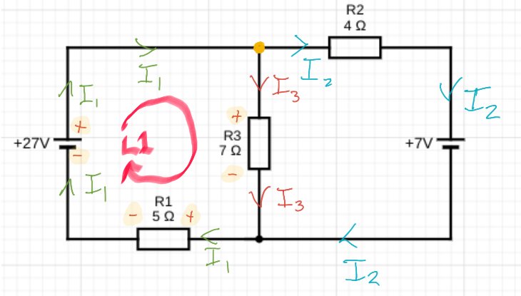
Going around loop L1 in the direction shown by the arrow:

• The emf 27 V will be positive as the potential increases (as we are moving from – to +).
• I₃R₃ will be negative as the potential decreases (as we are moving from + to -).
• I₁R₁ will be negative as the potential decreases (as we are moving from + to -).

This gives us:

Applying Kirchhoff’s Second Law (Part 2 of 2)

Going around Loop L2 we find that:

• The emf 7 V will be positive as the potential increases (as we are moving from – to +).
• I₂R₂ will be positive as the potential increases (as we are moving from – to +).
• I₃R₃ will be negative as the potential decreases (as we are moving from + to -).

This gives us:

The rest is history algebra

Going through a rather involved process of using simultaneous equations for solving for I₁, I₂ and I₃ . . .

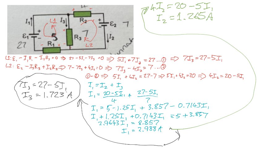
(NB There’s probably a quicker way than the way I chose, but I got there in the end and that’s the important thing. AND I guessed the direction of I₂ correctly. *Pats himself on the back*).

Conclusion

Kirchhoff’s Laws: I hope you give them a spin, whether or not you decide to use the procedure outlined above 🙂