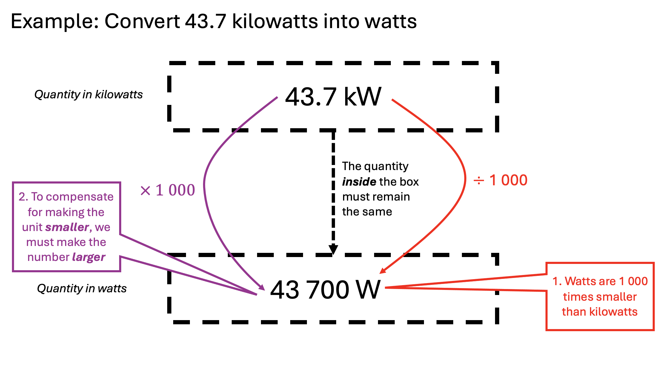
As I have written before, many students struggle with unit conversions. The Porter Method helps students’ understanding by making the process explicit.
Using the Porter Method to explain the mysteries of unit conversions
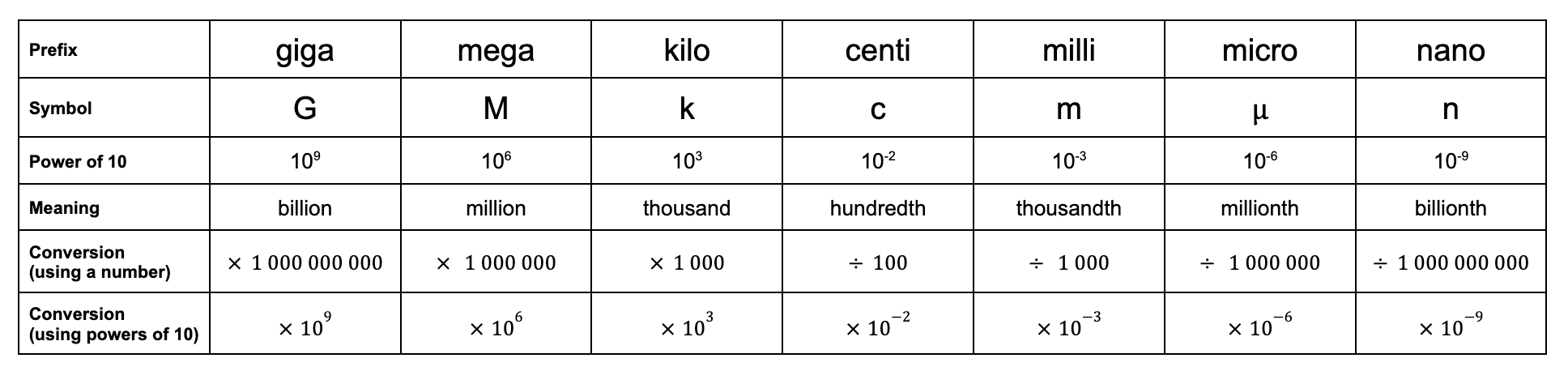
As of the time of writing, GCSE Science (2015 specification) students are expected to know the SI unit prefixes from giga- to nano-.
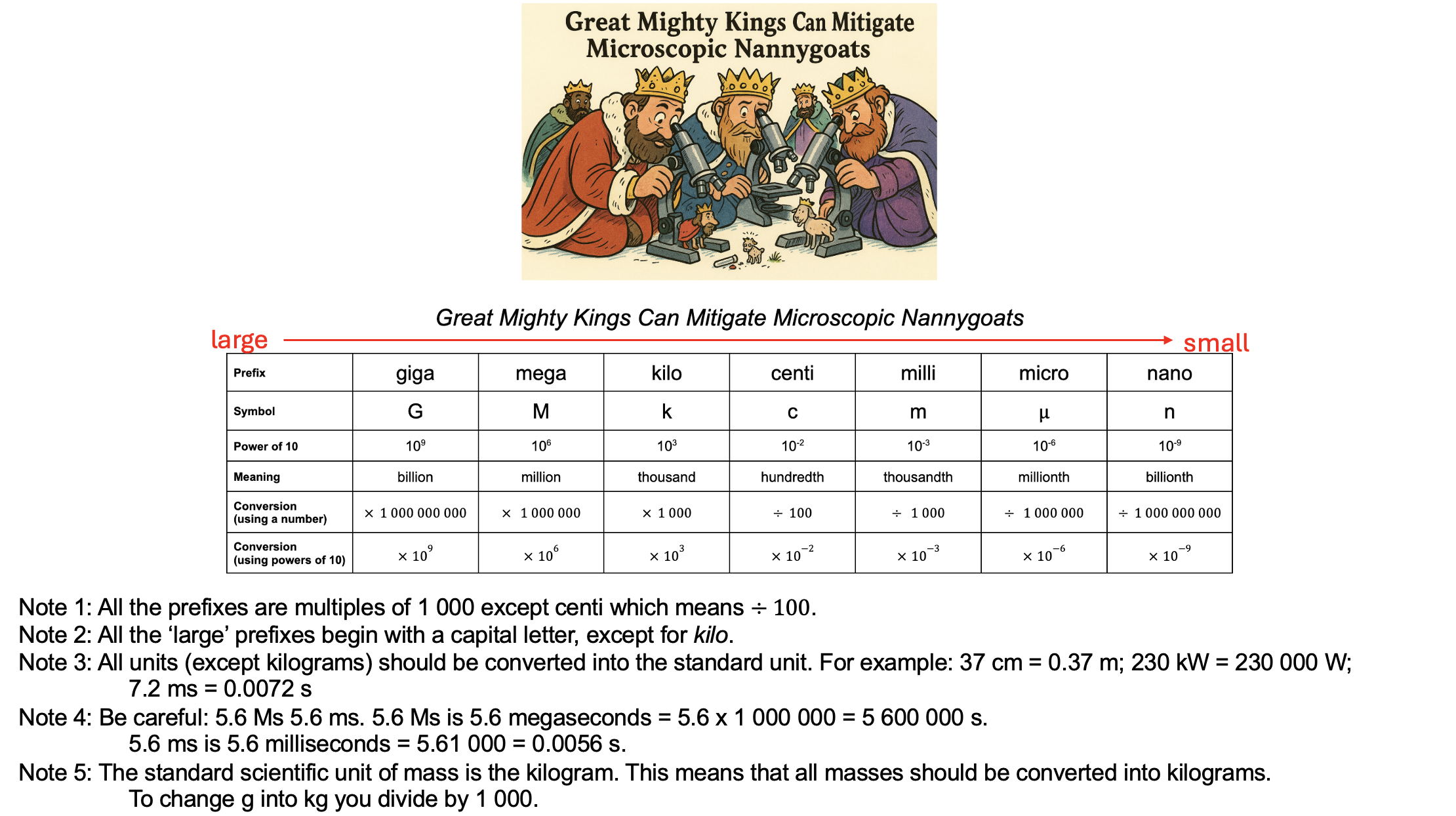
I suggest the following mnemonic:
A mnemonic for memorising the SI unit prefixes needed for GCSE
Choosing a mnemonic can be difficult because ‘mega’, ‘milli’ and ‘micro’ all begin with m, and even the first two letters of ‘milli’ and ‘micro’ are both ‘mi’. The mnemonic about helps students remember the difference between ‘milli’ and ‘micro’ by using ‘microscopic’ to help.
If you think this approach will be useful for your students, the Powerpoint is attached.
Enjoy!
PS You can find more of my thoughts on the SI system here
The philosopher John Stuart Mill (1806-1873) offers an intriguing system for classifying misconceptions (or ‘fallacies’ as he terms them) that could be useful for teachers in understanding many of the misconceptions and preconceptions that our students hold.
My own thoughts on this issue have been profoundly shaped by the ‘Resources Framework‘ as presented by authors such as Andrea di Sessa, David Hammer, Edward Redish and others. What follows is not a rejection of this approach but rather an exploration of whether Mill’s work offers some relevant insights. My thought is that it quite possibly might; after all, it has happened before . . .
The authors, however, did not use or refer to Mill’s system of logic in developing the programs or in formulating their theory of instruction. They didn’t discover parallels between their theory of instruction and Mill’s logic until after they had finished writing the bulk of ‘Theory of Instruction’. The discovery occurred when they were writing a chapter on theoretical issues. In their search for literature relevant to their philosophical orientation, they came across Mill’s work and were shocked to discover that they had independently identified all the major patterns that Mill had articulated. ‘Theory of Instruction’ (1982) even had parallel principles to the methods in ‘A System of Logic’ (1843)
Engelmann and Carnine 2013: Chapter 2
Mill’s system for classifying fallacies
In A System of Logic (1843), Mill argues that
Indifference to truth can not, in and by itself, produce erroneous belief; it operates by preventing the mind from collecting the proper evidences, or from applying to them the test of a legitimate and rigid induction; by which omission it is exposed unprotected to the influence of any species of apparent evidence which offers itself spontaneously, or which is elicited by that smaller quantity of trouble which the mind may be willing to take.
Mill 1843: Book V Chap 1
Mill is saying that we don’t believe false things because we want to, but because there are mechanisms preventing our minds from duly noting and weighing the myriad evidences from which we construct our beliefs about the world by the process of induction.
He suggests that there are five major classes of fallacies:
A priori fallacies;
Fallacies of observation;
Fallacies of generalisation;
Fallacies of ratiocination; and
Fallacies of confusion
Erroneous arguments do not admit of such a sharply cut division as valid arguments do. An argument fully stated, with all its steps distinctly set out, in language not susceptible of misunderstanding, must, if it be erroneous, be so in some one of these five modes unequivocally; or indeed of the first four, since the fifth, on such a supposition, would vanish. But it is not in the nature of bad reasoning to express itself thus unambiguously.
Mill 1843: Book V Chap 1
Mill is saying that invalid inferences, by their very nature, are ‘messier’ and harder to classify than correct inferences. However, they must all fit into the five categories outlined above. Actually, they are more likely to fit into the first four categories since clear and unambiguous use of language and terms would tend to eliminate fallacies of confusion as a matter of course.
What is an a priori fallacy?
In philosophy, a priori means knowledge derived from theoretical deduction rather than from empirical observation or experience.
Mill says that a priori fallacies (which he also calls fallacies of simple observation) are
those in which no actual inference takes place at all; the proposition (it cannot in such cases be called a conclusion) being embraced, not as proved, but as requiring no proof; as a self-evident truth.
Mill 1843: Book V Chap 3
In other words, an a priori fallacy is an idea whose truth is accepted on its face value alone; no evidence or justification of its truth is needed. An example from physics education might be ideas such as ‘heavy objects fall’ or ‘wood floats’. Some students accept these as obvious and self-evident truths: there is no need to consider ideas such as weight and resultant force or density and upthrust because these are ‘brute facts’ about the world that admit of no further explanation. This a case of mislabelling subjective facts as objective facts.
Falling is a location-specific behaviour: objects on Earth will indeed tend to accelerate downwards towards the centre of the Earth: this is a subjective fact which is dependent on the location of the object rather than an objective fact about the behaviour of all objects everywhere (although we could, of course, argue that falling is indeed an objective fact about objects which are subject to the influence of gravitational fields). Equally, floating is not a phenomenon restricted to the interaction between wood and water: many woods will sink in low density oils. ‘Wood floats‘ is not an objective fact about the universe but rather a subjective fact about the interaction of wood with a certain liquid.
This may be why some students are incurious about certain phenomena because they regard them as trivial and obvious rather than manifestations of the inner workings of the universe.
Mill lists many other examples of the a priori fallacy, but his examples are drawn from the history of science and philosophy, and so are of less direct relevance to the science classroom, with the possible exception of the two following examples:
Humans tend to default to the assumption that any phenomenon must necessarily have only a single cause; in other words, we assume that a multiplicity of causes is impossible. We are protected from this version of the a priori fallacy by the guard rail of the scientific method. For a complete understanding of a phenomenon, we look at the effect of one independent variable at a time whilst controlling other possible variables.
There remains one a priori fallacy or natural prejudice, the most deeply-rooted, perhaps, of all which we have enumerated; one which not only reigned supreme in the ancient world, but still possesses almost undisputed dominion over many of the most cultivated minds … This is, that the conditions of a phenomenon must, or at least probably will, resemble the phenomenon itself … the natural prejudice which led people to assimilate the action of bodies upon our senses, and through them upon our minds, to the transfer of a given form from one object to another by actual moulding.
Mill 1843: Book V Chap 3
I think that this tendency might be the one in play with the difficulties that many students have with understanding how images are formed: they think that an image is an evanescent ‘clone’ of the object that is being imaged rather than being an artefact of the light rays reflected or emitted from the object. This also might help explain why students find explaining the colour changes produced by looking at an object through a colour filter or illuminating it with coloured light difficult: they assume that colour is an essential unalterable property that adheres to the object and cannot be changed without changing the object.
We’ll continue this exploration of Mill’s classification of misconceptions in later posts.
References
Engelmann, S., & Carnine, D. (2013). Could John Stuart Mill Have Saved Our Schools? Attainment Company, Inc.
Mill, J. S. (1843). A System of Logic. Collected Works.
It is a truth which is by no means universally acknowledged, but one of which I hope shortly to persuade the reader, that introducing speed to 11-14 year-old students as speed=distance÷time or s=d ÷ t is not the most pedagogically effective approach.
This may initially seem like perverse idea since surely s = d ÷ t and s × t = d are mathematically equivalent expressions? They are, but it is my contention that many students find expressions of the format s = d ÷ t more cognitively demanding that s×t=d. This is because many students struggle with the concept of inverse relationships, particularly those involving multiplication and division.
[Researchers have] suggested that multiplicative concepts may be more difficult to acquire than additive ones, and speculated that although addition and subtraction concepts and procedures extend to multiplication and division, the latter also include unique aspects unrelated to addition and subtraction.
Robinson and LeFevre 2012: 426
In short, many students can handle solving problems such as a + b = c where (say) the numerical values of b and c are known. This can be solved by performing the operation a + b – b = c – b leading to a = c – b and hence a solution to the problem. However, students — and many adults(!) — find solving a similar problem of the format a=b÷c much more problematic, especially in cases when b÷c is not a simple integer.
Compounding students’ inability to utilise multiplicative structures, is their failure to recognise the isomorphism between proportion problems. Another possible reason is that a reluctance or inability to deal with the non-integer relationships (‘avoidance of fractions’), coupled with the high processing loads involved, seems to be the likely cause of this error
Singh 2000: 595
The problem with the s=d÷t format
In this analysis, we will assume that a direct calculation of s when d and t are known is trivial. The problem with the s=d÷t format is that it may require students to apply two problem solving procedures which, to the novice learner, have highly dissimilar surface features and whose underlying isomorphism is, therefore, hidden from them.
To find d if s and t are known, they need to multiply both sides by t (see Example 1).
To find t if s and d are known, they need to divide both sides by s and then multiply both sides by t (see Example 2)
Example 1
Example 2
(For more on using the ‘FIFA’ mnemonic for calculations, click on this link.)
Easing cognitive load with the s x t = d format
As above, we will assume that a direct calculation of d when s and t are known is trivial. What happens when we need to find s and t, given that they are the only unknown quantities?
If t and d are known, then we can find s by dividing both sides by t (see Example 3).
If s and t are known, then we can find t by dividing both sides s (see Example 4).
Example 3
Example 4
Examples 3 and 4 have highly similar surface features as well as a deeper level isomorphism and allow a commonality of approach which I think is immensely helpful for novice learners.
Robinson and LeFevre (2012: 411) call this type of operation ‘the inversion shortcut’ and argue (for a different context than the one presented here) that:
In three-term problems such as a × b ÷ b, the knowledge that b ÷ b = 1, combined with the associative property of multiplication, allows solvers to implement an inversion shortcut on problems such as 4×24÷24. The computational advantage of using the inversion shortcut is dramatic, resulting in greatly reduced solution times and error rates relative to a left-to-right solution procedure. […] Such knowledge of how inverse operations relate in a variety of circumstances forms the basis for understanding and manipulating algebraic expressions, an important mathematical activity for adolescents
Conclusion
I think there is a strong case to be made for this mode of presentation to be applied to a wider range of physics contexts for 11-16 year-old students such as:
Power, so that the definition of power is initially presented as P × t = E or P × t = W; that is to say, we define power as the energy transferred in one second.
Density, so that ρ × V = m; that is to say, we define density as mass of 1 m3 or 1 cm3.
Pressure, so that the definition of pressure is initially presented as p × A = F; that is to say, we define pressure as the force exerted on an area of 1 metre squared.
Acceleration, so that a × t = Δv; that is to say, we define acceleration as the change in velocity produced in one second.
Please feel free to leave a comment
References
Robinson, K. M., & LeFevre, J. A. (2012). The inverse relation between multiplication and division: Concepts, procedures, and a cognitive framework. Educational Studies in Mathematics, 79(3), 409-428.
Singh, P. (2000). Understanding the concepts of proportion and ratio among grade nine students in Malaysia. International Journal of Mathematical Education in Science and Technology, 31(4), 579-599.
I recently made a bit of a mess of teaching the topic of gears by trying to ‘wing it’ with insufficient preparation. To avoid my — and possibly others’ — future blushes, I thought I would compile a post summarising my interpretation of what students need to know about gears for AQA GCSE Physics.
I am going to include some handy gifs and a clean, un-annotated Google Jamboard (my favoured medium for lessons).
Any continuing errors, omissions or misconceptions are entirely my own fault.
‘A simple gear system can be used to transmit the rotational effect of a force’ [AQA 4.5.4]
A gear is a wheel with teeth that can transmit the rotational effect of a force.
For example, in the gear train shown above, the first gear (A) is turned by a motor (green dot shown below). The moment (rotational effect) is passed via the interlocking teeth to gear B and so on down the chain to gear E. It is also worth pointing out that gear A has a clockwise moment but gear B has an anticlockwise moment. The direction alternates as we move down the chain. It takes a gear train of five gears to transmit the clockwise moment from gear A to gear E.
Gears A-E are all equal in size with the same number of teeth and, consequently, the moment does not change in magnitude as it passes down the chain (although, as noted above, it does change direction from clockwise to anticlockwise).
‘Students should be able to explain how gears transmit the rotational effect of forces’ [AQA 4.5.4]
Part 1: A reduction gear arrangement
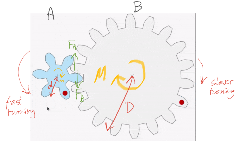
The driving gear (coloured blue) is smaller and has 6 teeth compared with the large gear’s 18 teeth. This is called a reduction gear arrangement.
A reduction gear arrangement does two things:
It slows down the speed of rotation. You may notice that the large gear turns only one for each three turns of the small gear.
The larger gear exerts a larger moment than the smaller gear. This is because the distance from the centre to the edge is larger for the grey gear.
The blue gear A exerts a force FA on gear B. By Newton’s Third Law, gear B exerts an equal but opposite force FB on gear A. Let’s take the magnitude of both forces to be F.
The anticlockwise moment exerted by gear A is given by m = F x d. The clockwise moment exerted by gear B is given by M=F x D. Since D > d then M > m.
A reduction gear arrangement is typically used in devices like an electric screwdriver. The electric motor in the device produces only a small rotational moment m but a large moment M is needed to turn the screws. The reduction gear produces the large moment M required.
Part 2: The overdrive arrangement
What happens when the driver gear is larger and has a greater number of teeth than the driven gear? This is called an overdrive arrangement.
The example we are going to look at is the arrangement of gears on a bicycle.
Here the driver gear (on the left) is linked via a chain to the smaller driven gear on the right. This means that the anticlockwise moment of the first gear is transmitted directly to the second gear as an anticlockwise moment. That is to say, the direction of the moment is not reversed as it is when the two gears are directly linked by interlocking teeth.
In the example shown, the big gear A turns only once for each four turns completed by the smaller gear B. Let’s assume that gear A exerts a force F on the chain so that the chain exerts an identical force F on gear B. Since D > d, this means that M > m so that the arrangement works as a distance multiplier rather than a force multiplier. This is, of course, excellent if we are riding at speed along a horizontal road. However, if we encounter an upward incline we may wish to — using the gear changing arrangement on the bike — swap the small gear B with one with a larger value of d. This would have the happy effect of increasing the magnitude of m so as to make it slightly easier to pedal uphill.
Circuit diagrams can be seen either as pictures or abstractions but it is clear that pupils often find it hard to recognise the circuits in the practical situation of real equipment. Moreover, Caillot found that students retain from their work with diagrams strong images rather than the principles they are intended to establish. The topological arrangement of a diagram or a drawing presents problems for pupils which are easily overlooked. It seems that pupils’ spatial abilities affect their use of circuit diagrams: they sometimes do not regard as identical several circuits, which, though identical, have been rotated so as to have a different spatial arrangement. […] Niedderer found that pupils, when asked whether a circuit diagram would ‘work’ in practice, more often judged symmetrical diagrams to be functioning than non-symmetric ones.
Driver et al. (1994): 124 [Emphases added]
For the reasons outlined by Driver and others above, I think it’s a good idea to vary the way that we present circuit diagrams to students when teaching electric circuits. If students always see circuit diagrams presented so that (say) the cell is at the ‘top’ and ‘facing’ a certain way; or that they are drawn so that they are symmetrical (which is an aesthetic rather that a scientific choice), then they may well incorrectly infer that these and other ‘accidental’ features of our circuit diagrams are the essential aspects that they should pay the most attention to.
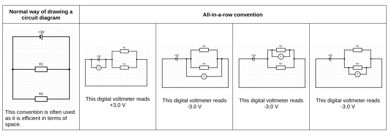
One ‘shake it up’ strategy is to redraw a circuit diagram using the ‘all-in-a-row’ convention.
If you arrange the real components in the ‘all-in-a-row’ arrangement, then a standard digital voltmeter has, what is in my opinion a regrettably underused functionality, that will show:
‘positive’ potential differences: that is to say, the energy added to the coulombs as they pass through a cell or the electromotive force; and
‘negative’ potential differences: that is to say, the energy removed from each coulomb as they pass through a resistor; these can be usefully referred to as ‘potential drops’
This can be shown on circuit diagrams as shown below/
In other words, the difference between the potential difference across the cell (energy being transferred into the circuit from the chemical energy store of the cell) is explicitly distinguished from the potential difference across the resistor (energy being transferred from the resistor into the thermal energy store of the surroundings). The all-in-a-row convention neatly sidesteps a common misconception that the potential difference across a cell is equal to the potential difference across a resistor: they are not. While they may be numerically equal, they are different in sign, as a consequence of Kirchoff’s Second Law. As I have suggested before, I think that this misconception is due to the ‘hidden rotation‘ built into standard circuit diagrams.
Potential divider circuits and the all-in-a-row convention
Although I am normally a strong proponent of the ‘parallel first heresy‘, I’ll go with the flow of ‘series circuit first’ in this post.
Diagrams 2 and 3 in the sequence show that the energy supplied to the coulombs (+1.5 V or 1.5 joules per coulomb) by the cell is transferred from the coulombs as they pass through the double resistor combination. Assuming that R1 = R2 then, as diagram 4 shows, 0.75 joules will be transferred out of each coulomb as they pass through R1; as diagram 5 shows, 0.75 joules will be transferred out of each coulomb as they pass through R2.
Parallel circuits and the all-in-a-row convention
I’ve written about using the all-in-a-row convention to help explain current flow in parallel circuits here, so I will focus on understanding potential difference in parallel circuit in this post.
Again, diagrams 2 and 3 in the sequence show that the positive 3.0 V potential difference supplied by the cell is numerically equal (but opposite in sign) to the negative 3.0 V potential drop across the double resistor combination. It is worth bearing in mind that each coulomb passing through the cell gains 3.0 joules of energy from the chemical energy store of the cell. Diagrams 4 and 5 show that each coulomb passing through either R1 or R1 loses its entire 3.0 joules of energy as it passes through that resistor. The all-in-a-row convention is useful, I think, for showing that each coulomb passes through just one resistor as it makes a single journey around the circuit.
Do we delve deeply enough into the actual physical mechanism of current flow through electrical conductors (in terms of charge carriers and electric fields) in our treatments for GCSE and A-level Physics? I must reluctantly admit that I am increasingly of the opinion that the answer is no.
Of course, as physics teachers we talk with seeming confidence of current, potential difference and resistance but — when push comes to shove — can we (say) explain why a bulb lights up almost instantaneously when a switch several kilometres away is closed when the charge carriers can be shown to be move at a speed comparable to that of a sedate jogger? This would imply a time delay of some tens of minutes between closing the switch and energy being transferred from the power source (via the charge carriers) to the bulb.
When students asked me about this, I tended to suggest one of the following:
“The electrons in the wire are repelling each other so when one close to the power source moves, then they all move”; or
“Energy is being transferred to each charge carrier via the electric field from the power source.”
However, to be brutally honest, I think such explanations are too tentative and “hand wavy” to be satisfactory. And I also dislike being that well-meaning but unintentionally oh-so-condescending physics teacher who puts a stop to interesting discussions with a twinkly-eyed “Oh you’ll understand that when you study physics at degree level.” (Confession: yes, I have been that teacher too often for comfort. Mea culpa.)
Sherwood and Chabay (1999) argue that an approach to circuit analysis in terms of a predominately classical model of electrostatic charges interacting with electric fields is very helpful:
Students’ tendency to reason locally and sequentially about electric circuits is directly addressed in this new approach. One analyzes dynamically the behaviour of the *whole* circuit, and there is a concrete physical mechanism for how different parts of the circuit interact globally with each other, including the way in which a downstream resistor can affect conditions upstream.
(Side note: I think the Coulomb Train Model — although highly simplified and applicable only to a limited set of “steady state” situations — is consistent with Sherwood and Chabay’s approach, but more on that later.)
Misconception 1: “The electrons in a conductor push each other forwards.”
On this model, the flowing electrons push each other forwards like water molecules pushing neighbouring water molecules through a hose. Each negatively charged electron repels every other negatively charged electron so if one free electron within the conductor moves, then the neighbouring free electrons will also move. Hence, by a chain reaction of mutual repulsion, all the electrons within the conductor will move in lockstep more or less simultaneously.
The problem with this model is that it ignores the presence of the positively charged ions within the metallic conductor. A conveniently arranged chorus-line of isolated electrons would, perhaps, behave analogously to the neighbouring water molecules in a hose pipe. However, as Sherwood and Chabay argue:
Averaged over a few atomic diameters, the interior of the metal is everywhere neutral, and on average the repulsion between flowing electrons is canceled by attraction to positive atomic cores. This is one of the reasons why an analogy between electric current and the flow of water can be misleading.
The flowing electrons inside a wire cannot push each other through the wire, because on average the repulsion by any electron is canceled by the attraction of a nearby positive atomic core (Diagram from Sherwood and Chabay 1999: 4)
Misconception 2: “The charge carriers move because of the electric field from the battery.”
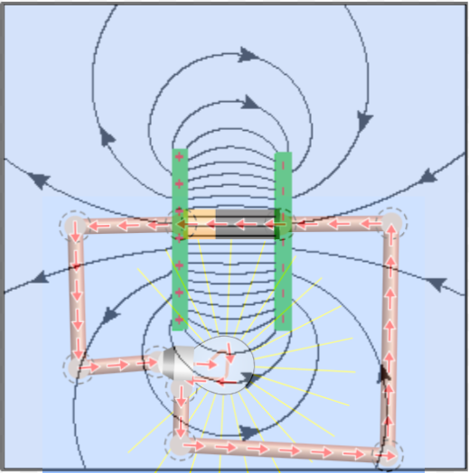
Let’s model the battery as a high-capacity parallel plate capacitor. This will avoid the complexities of having to consider chemical interactions within the cells. Think of a “quasi-steady state” where the current drawn from the capacitor is small so that electric charge on the plates remains approximately constant; alternatively, think of a mechanical charge transfer mechanism similar to the conveyor belt in a Van de Graaff generator which would be able to keep the charge on each plate constant and hence the potential difference across the plates constant (see Sherwood and Chabay 1999: 5).
A representation of the electric field around a single cell battery (modelled as a parallel plate capacitor)
This is not consistent with what we observe. For example, if the charge-carriers-move-due-to-electric-field-of the-battery model was correct then we would expect a bulb closer to the battery to be brighter than a more distant bulb; this would happen because the bulb closer to the battery would be subject to a stronger electric field and so we would expect a larger current.
A bulb closer to the battery is NOT brighter than a bulb further away from the battery (assuming negligible resistance in the connecting wires)
There is the additional argument if we orient the bulb so that the current flow is perpendicular to the electric field line, then there should be no current flow. Instead, we find that the orientation of the bulb relative to the electric field of the battery has zero effect on the brightness of the bulb.
There is no change of brightness as the orientation of the bulb is changed with respect to the electric field lines from the battery
Since we do not observe these effects, we can conclude that the electric field lines from the battery are not solely responsible for the current flow in the circuit.
Understanding the cause of current flow
If the electric field of the battery is not responsible on its own for the potential difference that causes a current to flow, where does the electric field come from?
Interviews reveal that students find the concept of voltage difficult or incomprehensible. It is not known how many students lose interest in physics because they fail to understand basic concepts. This number may be quite high. It is therefore astonishing that this unsatisfactory situation is accepted by most physics teachers and authors of textbooks since an alternative explanation has been known for well over one hundred years. The solution […] was in principle discovered over 150 years ago. In 1852 Wilhelm Weber pointed out that although a current-carrying conductor is overall neutral, it carries different densities of charges on its surface. Recognizing that a potential difference between two points along an electric circuit is related to a difference in surface charges [is the answer].
Härtel (2021): 21
We’ll look at these interesting ideas in part two.
[Note: this post edited 10/7/22 because of a rewritten part two]
I was “awoken from my dogmatic slumbers” on this topic (and alerted to Sherwood and Chabay’s treatment) by Youtuber Veritasium‘s provocative videos (see here and here).
When I was an A-level physics student (many, many years ago, when the world was young LOL) I found the derivation of the centripetal acceleration formula really hard to understand. What follows is a method that I have developed over the years that seems to work well. The PowerPoint is included at the end.
Step 1: consider an object moving on a circular path
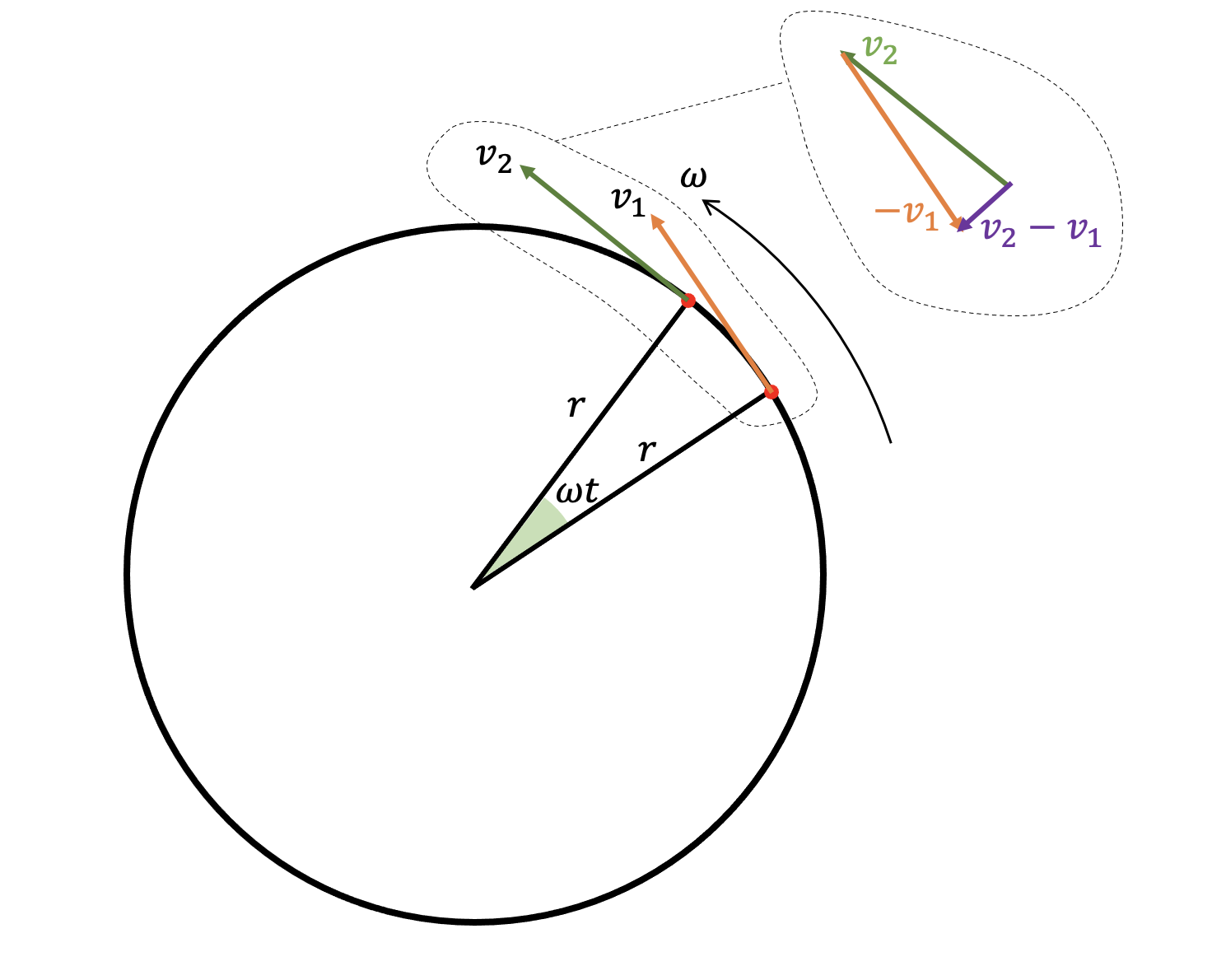
Let’s consider an object moving in circular path of radius r at a constant angular speed of ω (omega) radians per second.
The object is moving anticlockwise on the diagram and we show it at two instants which are time t seconds apart. This means that the object has moved an angular distance of ωt radians.
Step 2: consider the linear velocities of the object at these times
The linear velocity is the speed in metres per second and acts at a tangent to the circle, making a right angle with the radius of the circle. We have called the first velocity v1 and the second velocity at the later time v2.
Since the object is moving at a constant angular speed ω and is a fixed radius r from the centre of the circle, the magnitudes of both velocities will be constant and will be given by v = ωr.
Although the magnitude of the linear velocity has not changed, its direction most certainly has. Since acceleration is defined as the change in velocity divided by time, this means that the object has undergone acceleration since velocity is a vector quantity and a change in direction counts as a change, even without a change in magnitude.
Step 3a: Draw a vector diagram of the velocities
We have simply extracted v1 and v2 from the original diagram and placed them nose-to-tail. We have kept their magnitude and direction unchanged during this process.
Step 3b: close the vector diagram to find the resultant
The dark blue arrow is the result of adding v1 and v2. It is not a useful operation in this case because we are interested in the change in velocity not the sum of the velocities, so we will stop there and go back to the drawing board.
Step 3c switch the direction of velocity v1
Since we are interested in the change in velocity, let’s flip the direction of v1 so that it going in the opposite direction. Since it is opposite to v1, we can now call this -v1.
It is preferable to flip v1 rather than v2 since for a change in velocity we typically subtract the initial velocity from the final velocity; that is to say, change in velocity = v2 – v1.
Step 3d: Put the vectors v2 and (-v1) nose-to-tail
Step 3e: close the vector diagram to find the result of adding v2 and (-v1)
The purple arrow shows the result of adding v2 + (-v1); in other words, the purple arrow shows the change in velocity between v1 and v2 due to the change in direction (notwithstanding the fact that the magnitude of both velocities is unchanged).
It is also worth mentioning that that the direction of the purple (v2 –v1) arrow is in the opposite direction to the radius of the circle: in other words, the change in velocity is directed towards the centre of the circle.
Step 4: Find the angle between v2 and (-v1)
The angle between v2 and (-v1) will be ωt radians.
Step 5: Use the small angle approximation to represent v2-v1 as the arc of a circle
If we assume that ωt is a small angle, then the line representing v2-v1 can be replaced by the arc c of a circle of radius v (where v is the magnitude of the vectors v1 and v2 and v=ωr).
We can then use the familiar relationship that the angle θ (in radians) subtended at the centre of a circle θ = arc length / radius. This lets express the arc length c in terms of ω, t and r.
And finally, we can use the acceleration = change in velocity / time relationship to derive the formula for centripetal acceleration we a = ω2r.
Well, that’s how I would do it. If you would like to use this method or adapt it for your students, then the PowerPoint is attached.
Please Like or leave a comment if you find this useful 🙂
It is a truth universally acknowledged that student misconceptions about waves are legion. Why do so many students find understanding waves so difficult?
David Hammer (2000: S55) suggests that it may, in fact, be not so much a depressingly long list of ‘wrong’ ideas about waves that need to be laboriously expunged; but rather the root of students misconceptions about waves might be a simple case of miscategorisation.
Hammer (building on the work of di Sessa, Wittmann and others) suggests that students are predisposed to place waves in the category of object rather than the more productive category of event.
Thinking of a wave as an object imbues them with a notional permanence in terms of shape and location, as well as an intuitive sense of ‘weightiness’ or ‘mass’ that is permanently associated with the wave.
Looking at a wave through this p-prim or cognitive filter, students may assume that it can be understood in ways that are broadly similar to how an object is understood: one can simply look at or manipulate the ‘object’ whilst ignoring its current environment and without due consideration of its past or its future
For example, students who think that (say) flicking a slinky spring harder will produce a wave with a faster wave speed rather than the wave speed being dependent on the tension in the spring. They are using the misleading analogy of how an object such as a ball behaves when thrown harder rather than thinking correctly about the actual physics of waves.
A series of undulating events…
Hammer suggests that perhaps a more productive cognitive resource that we should seek to activate in our students when learning about waves is that of an event.
An event can be expected to have a location, a duration, a time of occurrence and a cause. Events do not necessarily possess the aspects of permanence that we typically associate with objects; that is to say, an event is expected to be a transient phenomenon that we can learn about by looking, yes, but we have to be looking at exactly the right place at the right time. We also cannot consider them independently of their environment: events have an effect on their immediate environment and are also affected by the environment.
If students think of waves as a series of events propagating through space they are less likely to imbue them with ‘permanent’ properties such as a fixed shape that can be examined at leisure rather than having to be ‘captured’ at one instant. Hammer suggests using a row of falling dominoes to introduce this idea, but you might also care to use this suggested procedure.
You can access an editable copy of the slides that follow in Google Jamboard format by clicking on this link.
Teaching Refraction Step 1: Breaking = bad waves
I like to start by anchoring the idea of changing wave speed in a context that students may be familiar with: waves on a beach. However, we should try and separate the general idea of an undulating water wave from that of a breaking wave. Begin by asking this question:
Give thirty seconds thinking time and then ask students to hold up either one or two fingers on 3-2-1-now! to show their preferred answer. (‘Finger voting’ is a great method for ensuring that every student answers without having to dig out those mini whiteboards).
The correct answer is, of course, the top diagram. This is because the bottom diagram shows a breaking wave.
Teaching Refraction Step 2: Why do waves ‘break’?
In short, because waves slow down as they hit the beach. The top part of the wave is moving faster than the bottom so the wave breaks up as it slides off the bottom part. In effect, the wave topples over because the bottom is moving more slowly than the top part.
The correct answer is ‘two fingers’
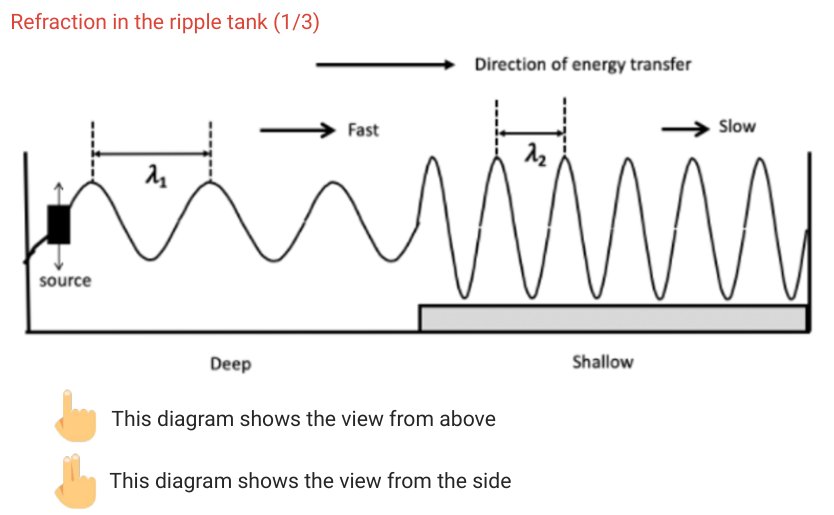
It is important that students appreciate that although the wavelength of the wave does change, the frequency of the wave does not. The frequency of the wave depends on the weather patterns that produced the wave in the deep ocean many hundreds or thousand of miles away. The slope of the beach cannot produce more or fewer waves per second. In other words, the frequency of a wave depends on its history, not its current environment.
All the beach can do is change the wave speed, not the wave frequency.
Teaching Refraction Step 3: the view from above
We can check our students’ understanding by asking them to comment or annotate a diagram similar to the one below.
Some good questions to ask — before the wavelength annotations are added — are:
Are we viewing the waves from above or from the side? (From above.)
Can we tell where the crests of the waves are? (Yes, where the line of foam are.)
Can we tell where the troughs of the waves are? (Yes, midway between the crests.)
Can we measure the wavelength of the waves? (Yes, the crest to crest distance.)
Can we tell if the waves are speeding up or slowing down as they reach the shore? (Yes, the waves are bunching together which suggests that slow down as they reach the shore.)
Teaching Refraction Step 4: Understanding the ripple tank
Physics teachers often assume that the operation and principles of a ripple tank are self-evident to students. In my experience, they are not and it is worth spending a little time exploring and explaining how a ripple tank works.
Teaching Refraction Step 5: the view from the side
Teaching Refraction Step 6: Seeing refraction in the ripple tank (1)
It’s a good idea to first show what happens when the waves hit the boundary at right angles; in other words, when the direction of travel of the waves is parallel to the normal line.
I like to add the annotations live with the class using Google Jamboard. (The questions can be covered with a blank box until you are ready to show them to the students.)
You can access an animated, annotable version of this and the other slides in this post in Google Jamboard format by clicking on this link.
Teaching Refraction Step 7: Seeing refraction in the ripple tank (2)
The next step is to show what happens when the water waves arrive at the boundary at an angle i; in other words, the direction of travel of the waves makes an angle of i degrees with the normal line.
Again, I like to add the annotations live using Google Jamboard.
It is a thing plainly repugnant . . . to Minister the Sacraments in a Tongue not understanded of the People.
Gilbert, Bishop of Sarum. An exposition of the Thirty-nine articles of the Church of England (1700)
How can we help our students understand physics better? Or, in more poetic language, how can we make physics a thing that is more ‘understanded of the pupils’?
Redish and Kuo (2015: 573) suggest that the Resources Framework being developed by a number of physics education researchers can be immensely helpful.
In summary, the Resources Framework models a student’s reasoning as based on the activation of a subset of cognitive resources. These ‘thinking resources’ can be classified broadly as:
Embodied cognition: these are simple, irreducible cognitive resources sometimes referred to as ‘phenomenological primitives’ or p-prims such as ‘if-resistance-increases-then-the-output-decreases‘ and ‘two-opposing-effects-can-result-in-a-state-of-dynamic-balance‘. They are typically straightforward and ‘obvious’ generalisations of our lived, everyday experience as we move through the physical world. Embodied cognition is perhaps summarised as our ‘sense of mechanism’.
Encyclopedic (ancillary) knowledge: this is a complex cognitive resource made of a large number of highly interconnected elements: for example, the concept of ‘banana’ is linked dynamically with the concept of ‘fruit’, ‘yellow’, ‘curved’ and ‘banana-flavoured’ (Redish and Gupta 2009: 7). Encyclopedic knowledge can be thought of as the product of both informal and formal learning.
Contextualisation: meaning is constructed dynamically from contextual and other clues. For example, the phrase ‘the child is safe‘ cues the meaning of ‘safe‘ = ‘free from the risk of harm‘ whereas ‘the park is safe‘ cues an alternative meaning of ‘safe‘ = ‘unlikely to cause harm‘. However, a contextual clue such as the knowledge that a developer had wanted to but failed to purchase the park would make the statement ‘the park is safe‘ activate the ‘free from harm‘ meaning for ‘safe‘. Contextualisation is the process by which cognitive resources are selected and activated to engage with the issue.
Using the Resources Framework for teaching
I have previously used aspects of the Resources Framework in my teaching and have found it thought provoking and helpful to my practice. However, the ideas are novel and complex — at least to me — so I have been trying to think of a way of conveniently organising them.
What follows in my ‘first draft’ . . . comments and suggestions are welcome!
The RGB Model of the Resources Framework
The RGB Model of the Resources Framework
The red circle (the longest wavelength of visible light) represents Embodied Cognition: the foundation of all understanding. As Kuo and Redish (2015: 569) put it:
The idea is that (a) our close sensorimotor interactions with the external world strongly influence the structure and development of higher cognitive facilities, and (b) the cognitive routines involved in performing basic physical actions are involved in even in higher-order abstract reasoning.
The green circle (shorter wavelength than red, of course) represents the finer-grained and highly-interconnected Encyclopedic Knowledge cognitive structures.
At any given moment, only part of the [Encyclopedic Knowledge] network is active, depending on the present context and the history of that particular network
Redish and Kuo (2015: 571)
The blue circle (shortest wavelength) represents the subset of cognitive resources that are (or should be) activated for productive understanding of the context under consideration.
A human mind contains a vast amount of knowledge about many things but has limited ability to access that knowledge at any given time. As cognitive semanticists point out, context matters significantly in how stimuli are interpreted and this is as true in a physics class as in everyday life.
Redish and Kuo (2015: 577)
Suboptimal Understanding Zone 1
A common preconception held by students is that the summer months are warmer because the Earth is closer to the Sun during this time of year.
The combination of cognitive resources that lead students to this conclusion could be summarised as follows:
Encyclopedic knowledge: the Earth’s orbit is elliptical
Embodied cognition: The closer to a heat source you are the warmer it is.
Both of these cognitive resources, considered individually, are true. It is their inappropriate selection and combination that leads to the incorrect or ‘Suboptimal Understanding Zone 1’.
To address this, the RF(RGB) suggests a two pronged approach to refine the contextualisation process.
Firstly, we should address the incorrect selection of encyclopedic knowledge. The Earth’s orbit is elliptical but the changing Earth-Sun distance cannot explain the seasons because (1) the point of closest approach is around Jan 4th (perihelion) which is winter in the northern hemisphere; (2) seasons in the northern and southern hemispheres do not match; and (3) the Earth orbit is very nearly circular with an eccentricity e of 0.0167 where a perfect circle has e = 0.
Secondly, the closer-is-warmer p-prim is not the best embodied cognition resource to activate. Rather, we should seek to activate the spread-out-is-less-intense ‘sense of mechanism’ as far as we are able to (for example by using this suggestion from the IoP).
Suboptimal Understanding Zone 2
Another common preconception held by students is all waves have similar properties to the ‘breaking’ waves on a beach and this means that the water moves with the wave.
The structure of this preconception could be broken down into:
Embodied cognition: if I stand close to the water on a beach, then the waves move forward to wash over my feet.
Encyclopaedic knowledge: the waves observed on a beach are water waves
Considered in isolation, both of these cognitive resources are unproblematic: they accurately describes our everyday, lived experience. It is the contextualisation process that leads us to apply the resources inappropriately and places us squarely in Suboptimal Understanding Zone 2.
The RF(RGB) Model suggests that we can address this issue in two ways.
Firstly, we could seek to activate a more useful embodied cognition resource by re-contextualising. For example, we could ask students to imagine themselves floating in deep water far from the shore: do the waves carry them in any particular direction or simply move them up or down as they pass by?
Secondly, we could seek to augment their encyclopaedic knowledge: yes, the waves on a beach are water waves but they are not typical water waves. The slope of the beach slows down the bottom part of the wave so the top part moves faster and ‘topples over’ — in other words, the water waves ‘break’ leading to what appears to be a rhythmic back-and-forth flow of the waves rather than a wave train of crests and troughs arriving a constant wave speed. (This analysis is over a short period of time where the effect of any tidal effects is negligible.)
Both processes try to ‘tug’ student understanding into the central, optimal zone.
Suboptimal Understanding Zone 3
Redish and Kuo (2015: 585) recount trying to help a student understand the varying brightness of bulbs in the circuit shown.
All bulbs are identical. Bulbs A and D are bright; bulbs B and C are dim.
The student said that they had spent nearly an hour trying to set up and solve the Kirchoff’s Law loop equations to address this problem but had been unsuccessful in accounting for the varying brightnesses.
Redish suggested to the student that they try an analysis ‘without the equations’ and just look at the problems in simpler physical terms using just the concept of electric current. Since current is conserved it must split up to pass through bulbs B and C. Since the brightness is dependent on the current, the smaller currents in B and C compared with A and D accounts for their reduced brightness.
When he was introduced to [this] approach to using the basic principles, he lit up and was able to solve the problem quickly and easily, saying, ‘‘Why weren’t we shown this way to do it?’’ He would still need to bring his conceptual understanding into line with the mathematical reasoning needed to set up more complex problems, but the conceptual base made sense to him as a starting point in a way that the algorithmic math did not.
Analysing this issue using the RF(RGB) it is plausible to suppose that the student was trapped in Suboptimal Understanding Zone 3. They had correctly selected the Kirchoff’s Law resources from their encyclopedic knowledge base, but lacked a ‘sense of mechanism’ to correctly apply them.
What Redish did was suggest using an embodied cognition resource (the idea of a ‘material flow’) to analyse the problem more productively. As Redish notes, this wouldn’t necessarily be helpful for more advanced and complex problems, but is probably pedagogically indispensable for developing a secure understanding of Kirchoff’s Laws in the first place.
Conclusion
The RGB Model is not a necessary part of the Resources Framework and is simply my own contrivance for applying the RF in the context of physics education at the high school level. However, I do think the RF(RGB) has the potential to be useful for both physics and science teachers.
Hopefully, it will help us to make all of our subject content more ‘understanded of the pupils’.
References
Redish, E. F., & Gupta, A. (2009). Making meaning with math in physics: A semantic analysis. GIREP-EPEC & PHEC 2009, 244.
Redish, E. F., & Kuo, E. (2015). Language of physics, language of math: Disciplinary culture and dynamic epistemology. Science & Education, 24(5), 561-590.
A huge thank you to everyone who has viewed, read or commented on one of my posts in 2021: whether you agreed or disagreed with my point of view, you are the people that make the work of writing this blog so enjoyable and rewarding.
The top 3 most-read posts of 2021 were:
1. What to do if your school has a batshit crazy marking policy
This particular post was written back in 2019 and it’s sobering to realise that it is still relevant enough that it was featured by @TeacherTapp in November 2021. As edu-blog writers will know, this unlooked for honour generates thousands of views — thanks, @TeacherTapp!
Note to schools: please, if you haven’t done so already, please please please sort out your marking policy and make sure it is workable and fit for purpose. It would seem that, even now, teachers are being made to mark for the sake of marking, rather than for any tangible educational benefit.
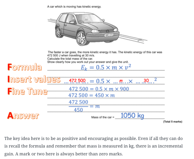
2. FIFA for the GCSE Physics Calculation Win!
The next post is one I am very proud of, even though FIFA is just a silly mnemonic to help students follow the “substitute-first-and-then-rearrange” method favoured by AQA mark schemes. Yes, FIFA did start life as a “mark-grubbing” dodge; however, somewhat to my own surprise, I found that the vast majority of students (LPAs included), can rearrange successfully if they substitute the numbers in first. Many other teachers have found the same thing as well — search #FIFAcalc on Twitter for some illustrative tweets from FIFAcalc’s biggest fans.
However, it is clear that the formula triangle method still has many adherents. I think this is unfortunate because: (a) they only work for a limited subset of formulas with the format y=mx; (b) they are a cognitive dead end that actively block students from accessing higher level STEM courses; and (c) as Ed Southall argues effectively, they are a form of procedural teaching rather than conceptual teaching.
3. Why does kinetic energy = 1/2mv^2?
This post is a surprise “sleeper” hit also dating from 2019. It outlines an accessible method for deriving the kinetic energy formula. From getting a respectable but niche 200 views per year in 2019 and 2020, in 2021 it shot up to over 3K views. What is very encouraging for me is that most of these views come from internet searches by individuals from a wide range of backgrounds and not just my fellow denizens of the online edu-Bubble!