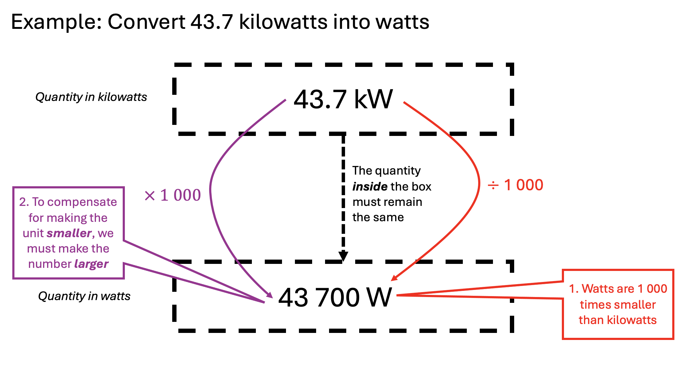
As I have written before, many students struggle with unit conversions. The Porter Method helps students’ understanding by making the process explicit.
Using the Porter Method to explain the mysteries of unit conversions
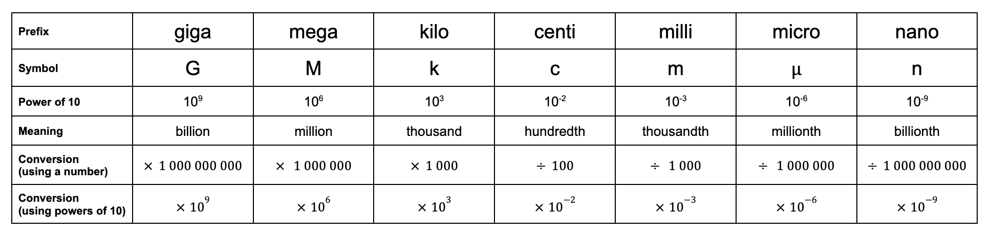
As of the time of writing, GCSE Science (2015 specification) students are expected to know the SI unit prefixes from giga- to nano-.
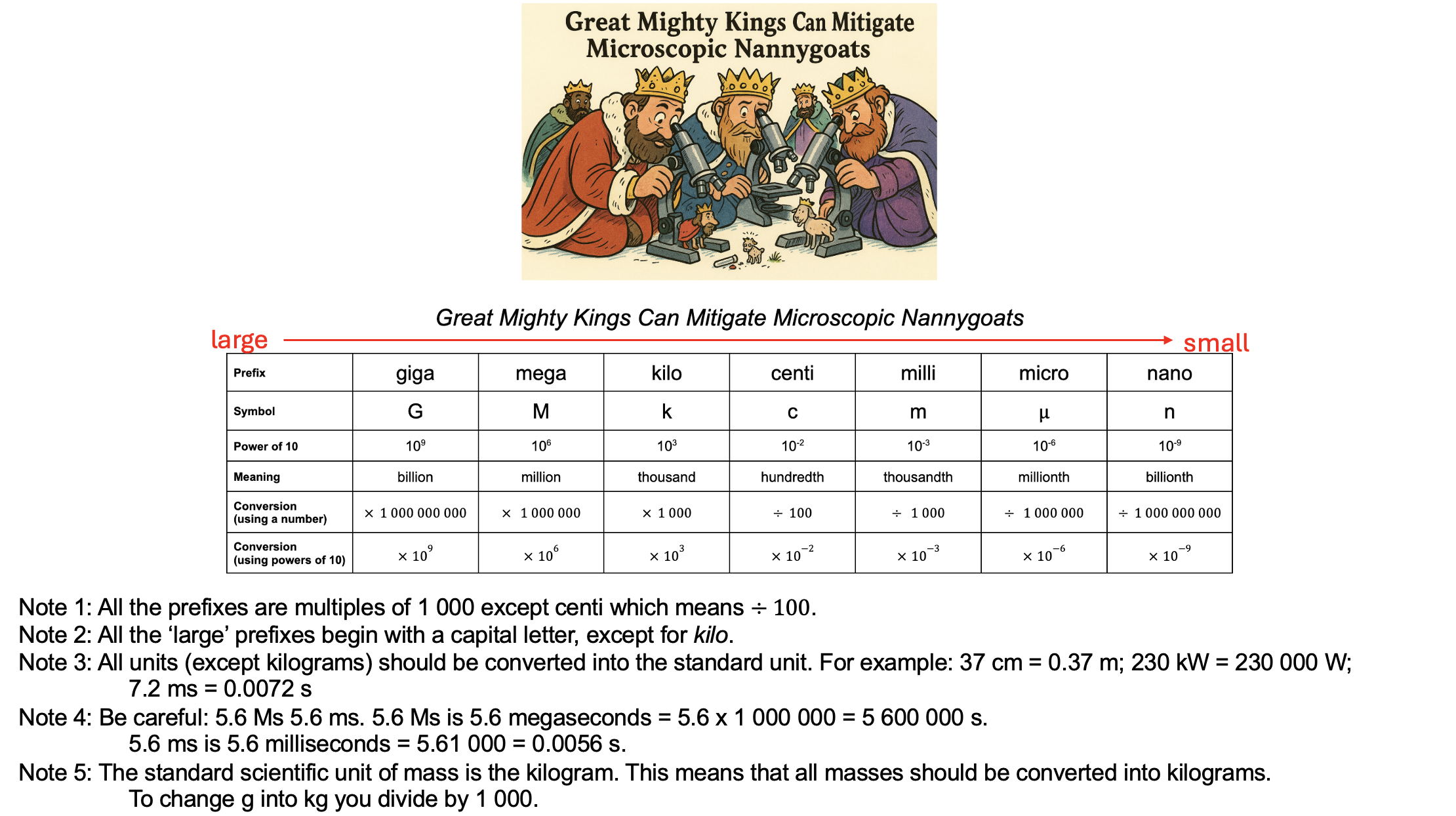
I suggest the following mnemonic:
A mnemonic for memorising the SI unit prefixes needed for GCSE
Choosing a mnemonic can be difficult because ‘mega’, ‘milli’ and ‘micro’ all begin with m, and even the first two letters of ‘milli’ and ‘micro’ are both ‘mi’. The mnemonic about helps students remember the difference between ‘milli’ and ‘micro’ by using ‘microscopic’ to help.
If you think this approach will be useful for your students, the Powerpoint is attached.
Enjoy!
PS You can find more of my thoughts on the SI system here
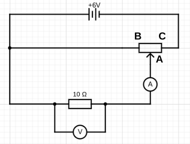
What is the worst circuit in the world? Many teachers think it is the one below.
This is the circuit that AQA (2018: 47) strongly suggest should be used to capture the data for plotting IV characteristics (aka current against potential difference graphs) for a fixed resistor, a filament lamp and a diode. The reasons why it is ‘the worst circuit in world’ were outlined in part one; and also some reasons why, nonetheless, schools teaching the 2016 AQA GCSE Physics / Combined Science specifications should (arguably) continue to use it.
The procedure outlined isn’t ‘perfect’ but works well using the equipment we have available and enables students to capture (and plot using a FREE Excel spreadsheet!) the data with only minor troubleshooting from the teacher.
Step the first: ‘These are the graphs you’re looking for.’
I find this required practical runs more smoothly if students have some awareness of what kind of graphs they are looking for. So, to borrow a phrase, I usually just tell ’em.
You can access an unannotated version of the slides on Google Jamboard and pdf below.
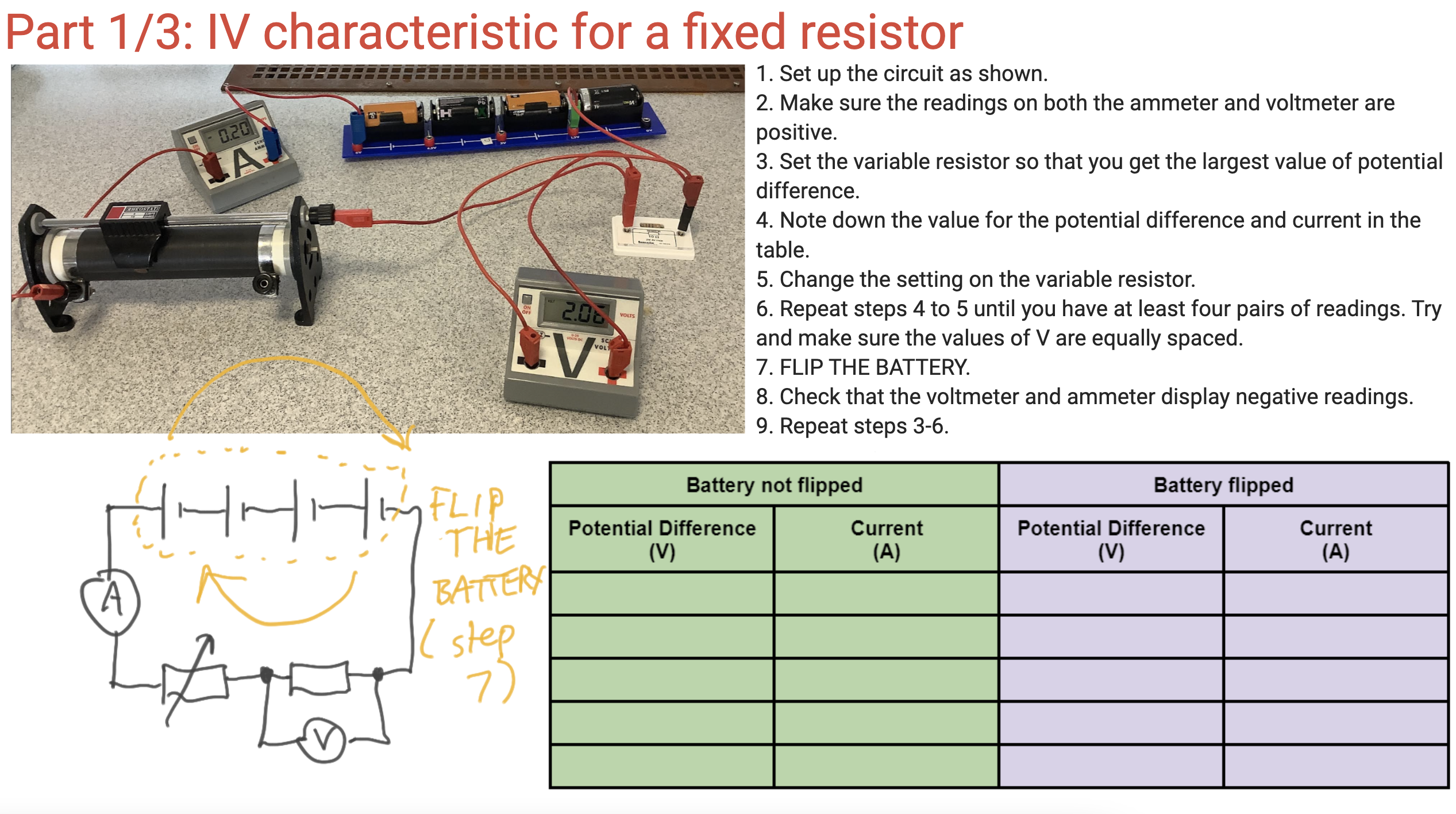
Step the second: capture the data for the fixed resistor
It is a continual source of amazement to me that students seem to find a photograph of a circuit easier to interpret than a nice, clean, minimalist circuit diagram, so for an easier life I present both.
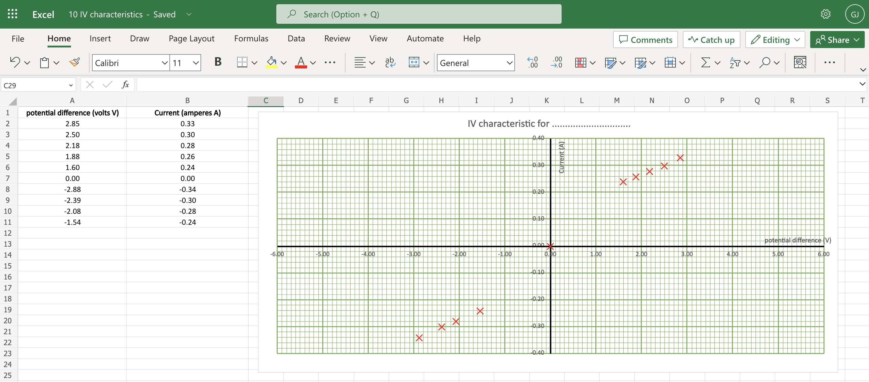
You can, if you have access to ICT, get the students to plot their results ‘live’ on an Excel spreadsheet (link below). I think this is excellent for helping to manage the cognitive demand on our students (as I have argued before here). Please note that I have not used the automated ‘line of best fit’ tools available on Excel as I think it is important for students to practice drawing lines of best fit — including, especially, curved lines of best fit (sorry, Maths teachers, in science there are such things as curved lines!)
Results for a fixed resistor from a typical group of students. These results are clearly consistent with a straight line of best fit going through the origin. However, they can be criticised for not being evenly spaced across the range — but this is a limitation of using the ‘worst circuit in the world’ and, happily(!), gives the students something to write about in their evaluation.
Step the second: capture the data for the filament lamp
In this circuit, we replaced the previous 0-16 ohm variable resistor with a 0 – 1000 ohm variable resistor paired with 2.5 V, 0.2 A filament lamp because the bulb has a resistance of about 60 ohms when run at 2.5 V and so the 0-16 ohm variable resistor is often ineffective. We allowed a maximum potential difference of just over 3.0 V to ‘over run’ the bulb so as to be sure of obtaining the ‘flattening’ of the graph. The method calls for very small adjustments of the variable resistor to obtain noticeable changes of brightness of the bulb. Note that the cells used in the photograph had seen many years of service with our physics department(!) and so were fairly depleted such that three of them were needed to produce a measly three volts; you would likely only need two ‘fresher’, ‘newer’ cells to achieve the same.
These are the results obtained by a typical student group. The results are clearly consistent with the elongated ‘S’ shaped curve predicted from theory. The results can be criticised for clustering, but this can be addressed by students in their evaluation of the experiment.
Step the third (sub-parts a and b): capturing the data for a diode
Results for diode captured by a group of students following the procedure outlined above.
And, by popular request, a copy of the PowerPoint below (although, trust me, I think Google Jamboard is superior when using ‘live’ in front of a class)
“The most miserable latch that’s ever been designed in the history of mankind or before.”
Astronaut Jack R. Lousma commenting on some equipment issues during the NASA Skylab 3 mission (July to September 1973), quoted in Cooper 1976: 41
What does the worst circuit that’s ever been designed in the history of humankind or before look like? Without further ado, here it is:
‘But wait,’ I hear you say, ‘isn’t this the circuit intended for obtaining the data for plotting current-potential difference characteristic curves as recommended by the AQA exam board in their GCSE Physics and GCSE Combined Science specifications?’ (AQA 2018: 47)
Sadly, it is indeed.
Why is ‘the standard test circuit’ a *bad* circuit?
The point of this required practical is to get several paired readings of potential difference across a component and the current through a component to enable us to plot a graph (aka ‘characteristic’) of current against potential difference. Ideally, we would like to start at 0.0 volts across the resistor and measure the current at (say) 1.0, 2.0, 3.0, 4.0, 5.0 and 6.0 volts. That is to say, we would like to treat the potential difference as the independent variable and adjust it in consistent, regular increments.
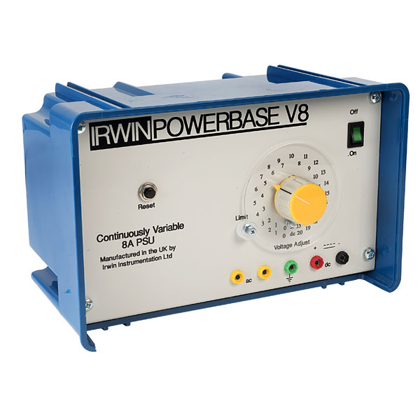
Now let’s say we use a typical school rheostat such as the one shown below as the variable resistor in series with the 10 ohm resistor. The two of them will behave as a potential divider circuit (see here and here for posts on this topic).
The resistance of the variable resistor can be varied between 0 and 16 ohms by moving the slider. When the slider is at A it will have the maximum resistance of 16 ohms and zero when it is at C, and in-between values at any other point.
A typical school rheostat. To use as a simple variable resistor, connect only terminals A and C into the circuit. (Please note: using terminals B and C will make it behave as a fixed resistor.)
When the slider is at C, the 10 ohm resistor gets the full potential difference from the supply and so the voltmeter will read 6.0 V and the ammeter will read (using I=V/R) 6.0 / 10 = 0.6 amps.
When the slider is at A, the total resistance of the circuit is 10 + 16 = 26 ohms so the ammeter reading (again using I=V/R) will be 6.0/26 = 0.23 amps. This means that the voltmeter reading (using V=IR) will be 0.23 x 10 = 2.3 volts.
This means that the circuit as presented will only allow us to obtain potential differences between a minimum of 2.3 V and a maximum of 6.0 V across the component by moving the slider between B and C, which is less than ideal.
‘It is a far, far better circuit that I build than I have ever built before…’
It is a far, far better thing that I do, than I have ever done.
Charles Dickens, ‘A Tale of Two Cities’
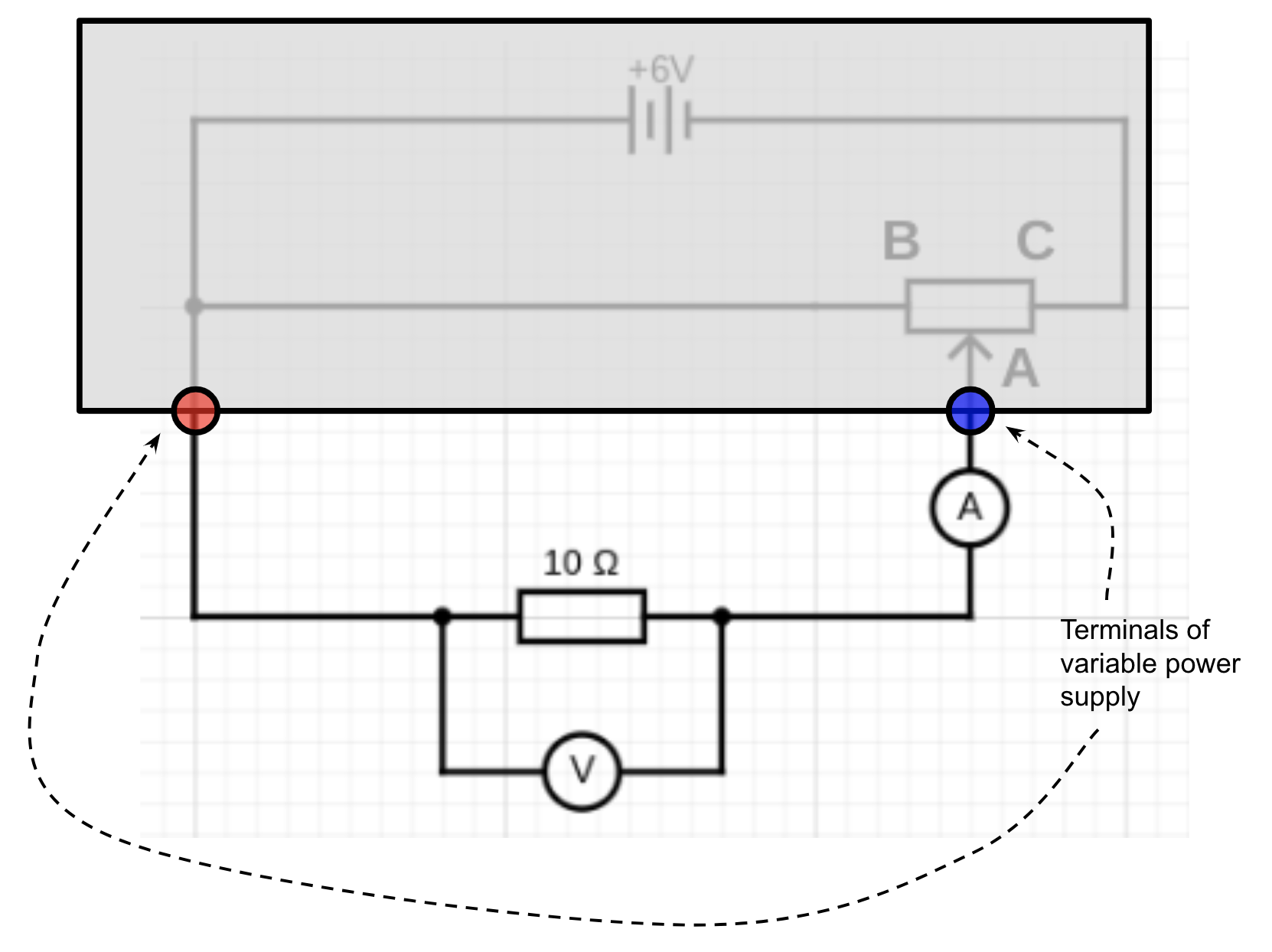
This circuit is a far better one for obtaining the data for a current-potential difference graph. This is because we can access the full 0.0 V to 6.0 V of the supply simply by adjusting the position of the rheostat slider. The rheostat is being used as a potential divider in this circuit rather than as a simple variable resistor.
When the slider is at B, the voltmeter will read 0.0 V and the current through the 10 ohm resistor will be 0.0 amps. A small movement of the slider from B towards C will increase the reading of the voltmeter to (say) 1.0 V and the ammeter would read 0.1 A. Further small movements of the slider will gradually increase the potential difference across the resistor until it reaches the full 6.0 V when the slider is at C.
A-level Physics students are expected to be able to use this circuit and enumerate its advantages over the ‘worst circuit in the world’.
And, to be fair, AQA do suggest a workaround that will allow GCSE student to side-step using ‘the worst circuit in the world’:
If a lab pack is used for the power supply this can remove the need for the rheostat as the potential difference can be varied directly. The voltage should not be allowed to get so high as to damage the components, check the rating of the components you plan to suggest your students use.
AQA 2018: 16
A ‘lab pack’ i.e. a power supply with a variable output potential difference
If this method is used, then in effect you would be using the ‘built in’ rheostat inside the power supply.
So why not use the superior potential divider circuit at GCSE?
The arguments in favour of using ‘the worst circuit in the world’ as opposed to the more fit for purpose potential divider circuit are:
The ‘worst circuit in the world’ is (arguably) conceptually easier than the potential divider circuit, especially if students have not studied series and parallel circuit before. This allows more freedom in sequencing when IV characteristics are taught.
A fuller range of potential differences can be accessed even using the ‘worst circuit in the world’ if the maximum value of the variable resistor is much larger than the resistance of the component. For example, if we used a 0 – 1 kilo-ohm variable resistor in series with the 10 ohm resistor then very fine adjustments of the variable resistor would allow a suitable range of potential difference to be applied across the component.
Students are often asked direct questions about the ‘worst circuit in world’.
Question from AQA Paper 1 (2021) where students who have used ‘the worst circuit in the world’ for their investigation would (imo) have an advantage over those that have not.
In the next post, I will outline how I introduce and teach this required practical — using, to my shame, ‘the worst circuit in the world’ — and also supply some useful resources.
It is a truth which is by no means universally acknowledged, but one of which I hope shortly to persuade the reader, that introducing speed to 11-14 year-old students as speed=distance÷time or s=d ÷ t is not the most pedagogically effective approach.
This may initially seem like perverse idea since surely s = d ÷ t and s × t = d are mathematically equivalent expressions? They are, but it is my contention that many students find expressions of the format s = d ÷ t more cognitively demanding that s×t=d. This is because many students struggle with the concept of inverse relationships, particularly those involving multiplication and division.
[Researchers have] suggested that multiplicative concepts may be more difficult to acquire than additive ones, and speculated that although addition and subtraction concepts and procedures extend to multiplication and division, the latter also include unique aspects unrelated to addition and subtraction.
Robinson and LeFevre 2012: 426
In short, many students can handle solving problems such as a + b = c where (say) the numerical values of b and c are known. This can be solved by performing the operation a + b – b = c – b leading to a = c – b and hence a solution to the problem. However, students — and many adults(!) — find solving a similar problem of the format a=b÷c much more problematic, especially in cases when b÷c is not a simple integer.
Compounding students’ inability to utilise multiplicative structures, is their failure to recognise the isomorphism between proportion problems. Another possible reason is that a reluctance or inability to deal with the non-integer relationships (‘avoidance of fractions’), coupled with the high processing loads involved, seems to be the likely cause of this error
Singh 2000: 595
The problem with the s=d÷t format
In this analysis, we will assume that a direct calculation of s when d and t are known is trivial. The problem with the s=d÷t format is that it may require students to apply two problem solving procedures which, to the novice learner, have highly dissimilar surface features and whose underlying isomorphism is, therefore, hidden from them.
To find d if s and t are known, they need to multiply both sides by t (see Example 1).
To find t if s and d are known, they need to divide both sides by s and then multiply both sides by t (see Example 2)
Example 1
Example 2
(For more on using the ‘FIFA’ mnemonic for calculations, click on this link.)
Easing cognitive load with the s x t = d format
As above, we will assume that a direct calculation of d when s and t are known is trivial. What happens when we need to find s and t, given that they are the only unknown quantities?
If t and d are known, then we can find s by dividing both sides by t (see Example 3).
If s and t are known, then we can find t by dividing both sides s (see Example 4).
Example 3
Example 4
Examples 3 and 4 have highly similar surface features as well as a deeper level isomorphism and allow a commonality of approach which I think is immensely helpful for novice learners.
Robinson and LeFevre (2012: 411) call this type of operation ‘the inversion shortcut’ and argue (for a different context than the one presented here) that:
In three-term problems such as a × b ÷ b, the knowledge that b ÷ b = 1, combined with the associative property of multiplication, allows solvers to implement an inversion shortcut on problems such as 4×24÷24. The computational advantage of using the inversion shortcut is dramatic, resulting in greatly reduced solution times and error rates relative to a left-to-right solution procedure. […] Such knowledge of how inverse operations relate in a variety of circumstances forms the basis for understanding and manipulating algebraic expressions, an important mathematical activity for adolescents
Conclusion
I think there is a strong case to be made for this mode of presentation to be applied to a wider range of physics contexts for 11-16 year-old students such as:
Power, so that the definition of power is initially presented as P × t = E or P × t = W; that is to say, we define power as the energy transferred in one second.
Density, so that ρ × V = m; that is to say, we define density as mass of 1 m3 or 1 cm3.
Pressure, so that the definition of pressure is initially presented as p × A = F; that is to say, we define pressure as the force exerted on an area of 1 metre squared.
Acceleration, so that a × t = Δv; that is to say, we define acceleration as the change in velocity produced in one second.
Please feel free to leave a comment
References
Robinson, K. M., & LeFevre, J. A. (2012). The inverse relation between multiplication and division: Concepts, procedures, and a cognitive framework. Educational Studies in Mathematics, 79(3), 409-428.
Singh, P. (2000). Understanding the concepts of proportion and ratio among grade nine students in Malaysia. International Journal of Mathematical Education in Science and Technology, 31(4), 579-599.
I recently made a bit of a mess of teaching the topic of gears by trying to ‘wing it’ with insufficient preparation. To avoid my — and possibly others’ — future blushes, I thought I would compile a post summarising my interpretation of what students need to know about gears for AQA GCSE Physics.
I am going to include some handy gifs and a clean, un-annotated Google Jamboard (my favoured medium for lessons).
Any continuing errors, omissions or misconceptions are entirely my own fault.
‘A simple gear system can be used to transmit the rotational effect of a force’ [AQA 4.5.4]
A gear is a wheel with teeth that can transmit the rotational effect of a force.
For example, in the gear train shown above, the first gear (A) is turned by a motor (green dot shown below). The moment (rotational effect) is passed via the interlocking teeth to gear B and so on down the chain to gear E. It is also worth pointing out that gear A has a clockwise moment but gear B has an anticlockwise moment. The direction alternates as we move down the chain. It takes a gear train of five gears to transmit the clockwise moment from gear A to gear E.
Gears A-E are all equal in size with the same number of teeth and, consequently, the moment does not change in magnitude as it passes down the chain (although, as noted above, it does change direction from clockwise to anticlockwise).
‘Students should be able to explain how gears transmit the rotational effect of forces’ [AQA 4.5.4]
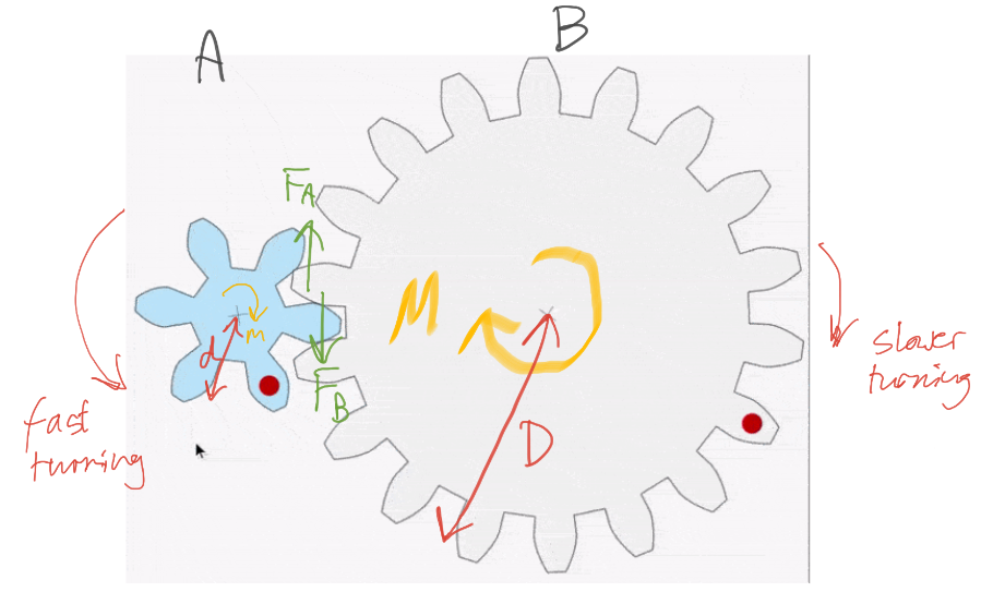
Part 1: A reduction gear arrangement
The driving gear (coloured blue) is smaller and has 6 teeth compared with the large gear’s 18 teeth. This is called a reduction gear arrangement.
A reduction gear arrangement does two things:
It slows down the speed of rotation. You may notice that the large gear turns only one for each three turns of the small gear.
The larger gear exerts a larger moment than the smaller gear. This is because the distance from the centre to the edge is larger for the grey gear.
The blue gear A exerts a force FA on gear B. By Newton’s Third Law, gear B exerts an equal but opposite force FB on gear A. Let’s take the magnitude of both forces to be F.
The anticlockwise moment exerted by gear A is given by m = F x d. The clockwise moment exerted by gear B is given by M=F x D. Since D > d then M > m.
A reduction gear arrangement is typically used in devices like an electric screwdriver. The electric motor in the device produces only a small rotational moment m but a large moment M is needed to turn the screws. The reduction gear produces the large moment M required.
Part 2: The overdrive arrangement
What happens when the driver gear is larger and has a greater number of teeth than the driven gear? This is called an overdrive arrangement.
The example we are going to look at is the arrangement of gears on a bicycle.
Here the driver gear (on the left) is linked via a chain to the smaller driven gear on the right. This means that the anticlockwise moment of the first gear is transmitted directly to the second gear as an anticlockwise moment. That is to say, the direction of the moment is not reversed as it is when the two gears are directly linked by interlocking teeth.
In the example shown, the big gear A turns only once for each four turns completed by the smaller gear B. Let’s assume that gear A exerts a force F on the chain so that the chain exerts an identical force F on gear B. Since D > d, this means that M > m so that the arrangement works as a distance multiplier rather than a force multiplier. This is, of course, excellent if we are riding at speed along a horizontal road. However, if we encounter an upward incline we may wish to — using the gear changing arrangement on the bike — swap the small gear B with one with a larger value of d. This would have the happy effect of increasing the magnitude of m so as to make it slightly easier to pedal uphill.
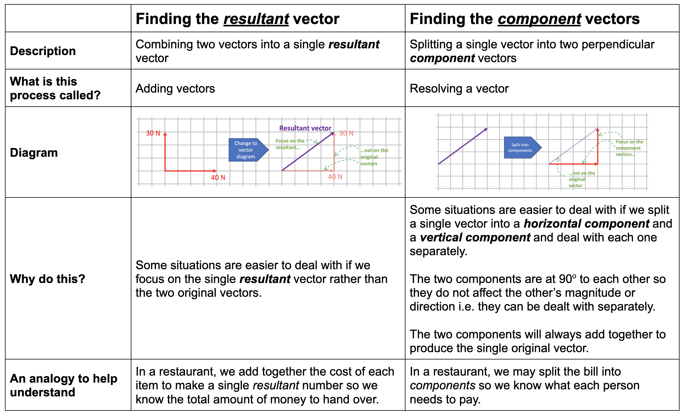
This post suggests some strategies for teaching vectors to 14-16 olds. In part 1 we looked at the idea of combining two vectors into one; that is to say, finding the resultant vector. In this part, we’re going to look at the inverse operation: splitting a single vector into two component vectors.
We’re going to use scale drawing rather than trigonometry since (a) this often leads to a more secure understanding; and (b) it is the expected method in the UK curriculum for 14-16 year olds.
What is a component vector?
A component vector is one of at least two vectors that will combine to give one single original vector. The component vectors are chosen so that they are mutually perpendicular. Because of this, they cannot affect each other’s magnitude and direction and so can be dealt with separately and independently; that is to say, we can choose to consider what effect the vertical component will have on its own without having to worry about what effect the horizontal component will have.
Introducing components as ‘the vector less travelled by’
Two roads diverged in a wood, and I—
I took the one less traveled by,
And that has made all the difference.

Robert Frost, 'The Road Less Travelled'
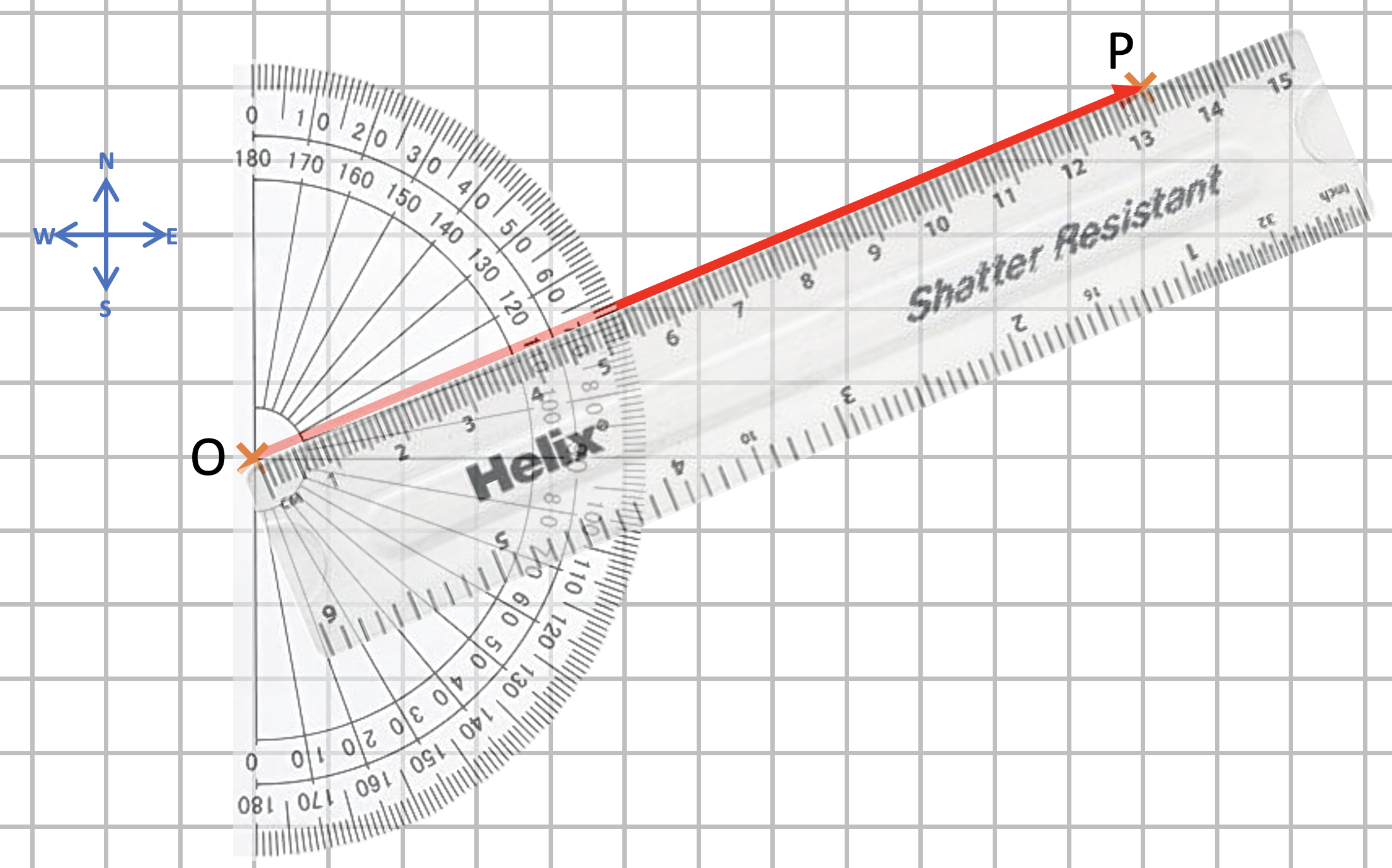
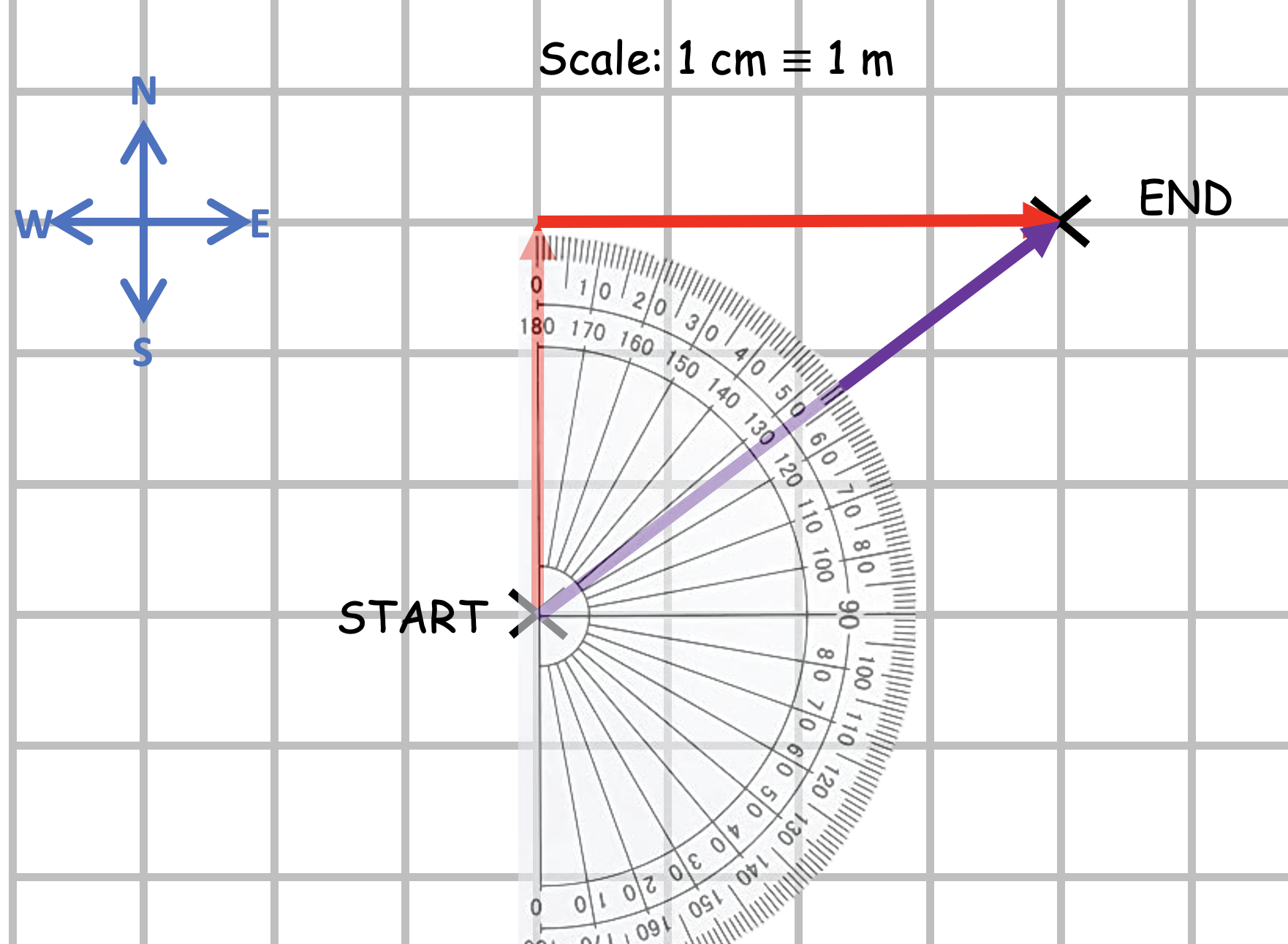
Let’s say we travelled a distance of 13 m from point O to point P on a compass bearing of 067 degrees (bear with me, I’m working with a slightly less familiar Pythagorean 3:4:5 triple here). This could be drawn as a scale diagram as shown below.
Could we analyse the displacement OP in terms of an eastward displacement and a northward displacement?
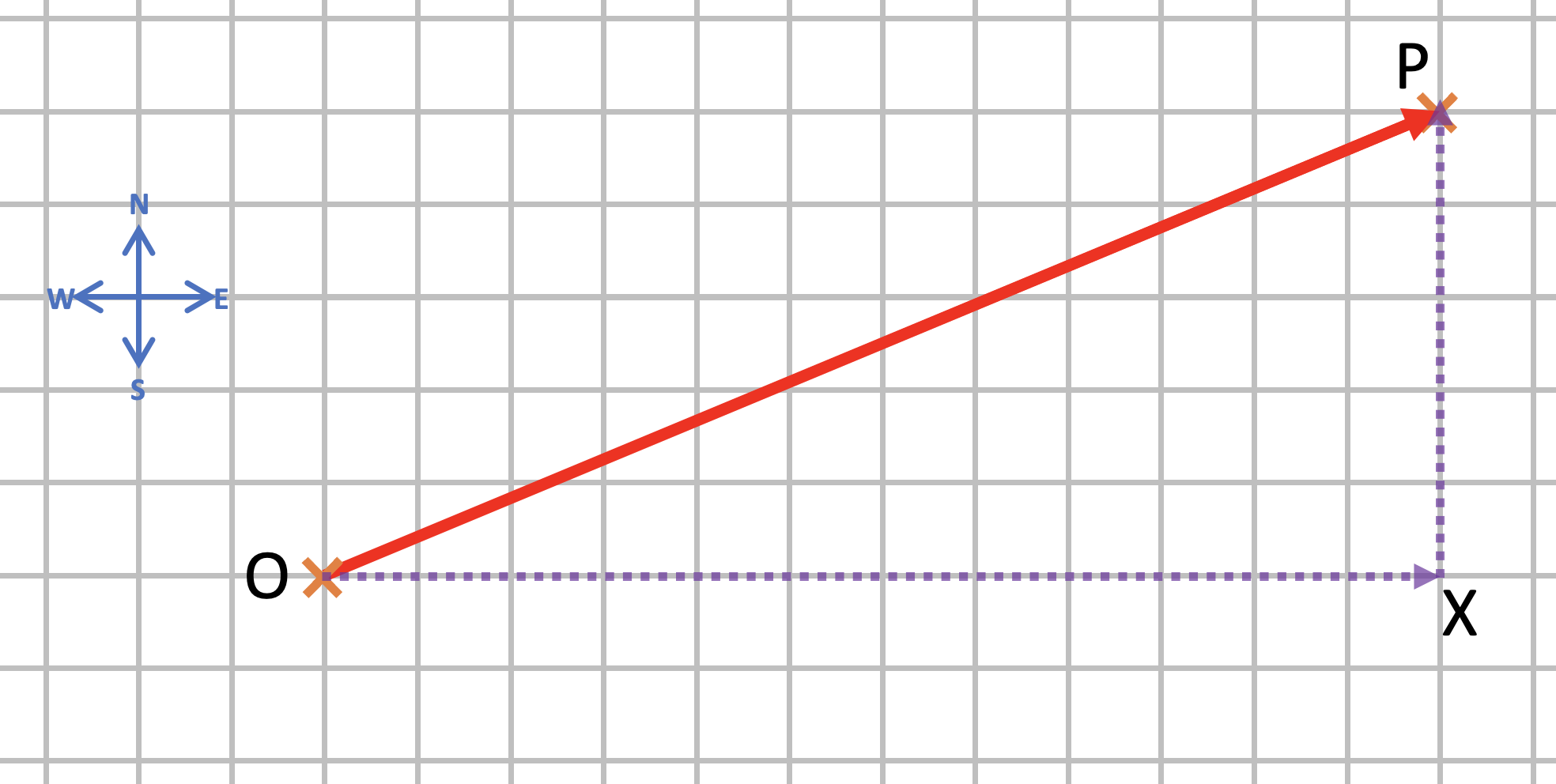
We can — as shown below.
The dotted line OX is the eastward (horizontal on our diagram) component of the displacement OP. It is drawn as a dotted line because it is (literally) the ‘road less travelled’. We did not walk along that road — and that’s why it is drawn as a dotted line — but we could have done.
But let’s say that we had, and that we had stopped when we reached the point marked X. And then we look around, and strike out northwards and walk the (vertical) ‘road less travelled called XP — and we end up at P.
So walking one road less travelled might, indeed, make ‘all the difference’ — but walking two roads less travelled does not.
To rewrite Robert Frost: We took the two roads less travelled by / And that has made NO difference.
But why should we wish to go the ‘long way around’, even if we still end up at P? Because it would allow us to work out the change in longitude and latitude. By moving from O to P we change our longitude by 12 metres and our latitude by 5 metres. (Don’t believe me? Count the squares on the diagram!)
We have resolved the 13 metre distance into two components: one eastward (horizontal) component of 12 metres and one northward component of 5 metres.
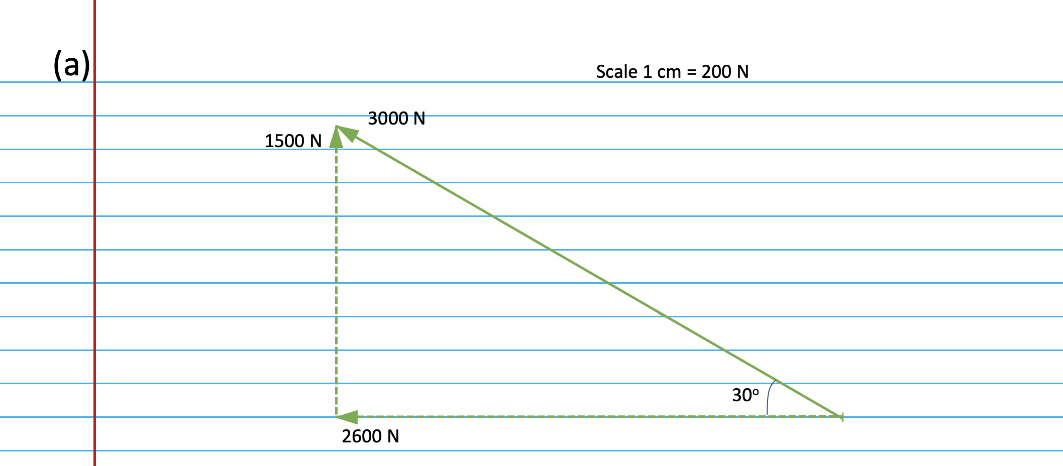
Using resolving a vector into components to solve problems
Circuit diagrams can be seen either as pictures or abstractions but it is clear that pupils often find it hard to recognise the circuits in the practical situation of real equipment. Moreover, Caillot found that students retain from their work with diagrams strong images rather than the principles they are intended to establish. The topological arrangement of a diagram or a drawing presents problems for pupils which are easily overlooked. It seems that pupils’ spatial abilities affect their use of circuit diagrams: they sometimes do not regard as identical several circuits, which, though identical, have been rotated so as to have a different spatial arrangement. […] Niedderer found that pupils, when asked whether a circuit diagram would ‘work’ in practice, more often judged symmetrical diagrams to be functioning than non-symmetric ones.
Driver et al. (1994): 124 [Emphases added]
For the reasons outlined by Driver and others above, I think it’s a good idea to vary the way that we present circuit diagrams to students when teaching electric circuits. If students always see circuit diagrams presented so that (say) the cell is at the ‘top’ and ‘facing’ a certain way; or that they are drawn so that they are symmetrical (which is an aesthetic rather that a scientific choice), then they may well incorrectly infer that these and other ‘accidental’ features of our circuit diagrams are the essential aspects that they should pay the most attention to.
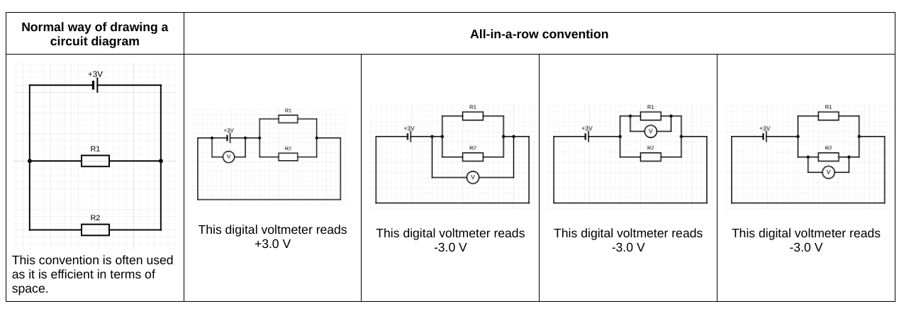
One ‘shake it up’ strategy is to redraw a circuit diagram using the ‘all-in-a-row’ convention.
If you arrange the real components in the ‘all-in-a-row’ arrangement, then a standard digital voltmeter has, what is in my opinion a regrettably underused functionality, that will show:
‘positive’ potential differences: that is to say, the energy added to the coulombs as they pass through a cell or the electromotive force; and
‘negative’ potential differences: that is to say, the energy removed from each coulomb as they pass through a resistor; these can be usefully referred to as ‘potential drops’
This can be shown on circuit diagrams as shown below/
In other words, the difference between the potential difference across the cell (energy being transferred into the circuit from the chemical energy store of the cell) is explicitly distinguished from the potential difference across the resistor (energy being transferred from the resistor into the thermal energy store of the surroundings). The all-in-a-row convention neatly sidesteps a common misconception that the potential difference across a cell is equal to the potential difference across a resistor: they are not. While they may be numerically equal, they are different in sign, as a consequence of Kirchoff’s Second Law. As I have suggested before, I think that this misconception is due to the ‘hidden rotation‘ built into standard circuit diagrams.
Potential divider circuits and the all-in-a-row convention
Although I am normally a strong proponent of the ‘parallel first heresy‘, I’ll go with the flow of ‘series circuit first’ in this post.
Diagrams 2 and 3 in the sequence show that the energy supplied to the coulombs (+1.5 V or 1.5 joules per coulomb) by the cell is transferred from the coulombs as they pass through the double resistor combination. Assuming that R1 = R2 then, as diagram 4 shows, 0.75 joules will be transferred out of each coulomb as they pass through R1; as diagram 5 shows, 0.75 joules will be transferred out of each coulomb as they pass through R2.
Parallel circuits and the all-in-a-row convention
I’ve written about using the all-in-a-row convention to help explain current flow in parallel circuits here, so I will focus on understanding potential difference in parallel circuit in this post.
Again, diagrams 2 and 3 in the sequence show that the positive 3.0 V potential difference supplied by the cell is numerically equal (but opposite in sign) to the negative 3.0 V potential drop across the double resistor combination. It is worth bearing in mind that each coulomb passing through the cell gains 3.0 joules of energy from the chemical energy store of the cell. Diagrams 4 and 5 show that each coulomb passing through either R1 or R1 loses its entire 3.0 joules of energy as it passes through that resistor. The all-in-a-row convention is useful, I think, for showing that each coulomb passes through just one resistor as it makes a single journey around the circuit.
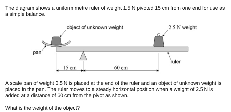
Many years ago, I was taught this compact and intuitive convention to show turning moments. I think it should be more widely known, as it not only is concise and powerful, but also meets the criterion of being an effective form of dual coding which is helpful for both GCSE and A-level Physics students.
Let’s look at an example question.
Let’s start by ‘annotating the hell’ out of the diagram.
We could take moments around any of the marked points A-E on the diagram. However, we’re going to take moments around B as it enables us to ignore the upward reaction force acting on the rule at B. (This force is not shown on the diagram.)
To indicate that we’re going to be considering the sum of the clockwise moments about point B, we use this intuitive notation:
If we consider the sum of anticlockwise moments about point B, we use this:
We lay out our calculations of the total clockwise and anticlockwise moments about B as follows.
We show that we are going to apply the Principle of Moments (the sum of clockwise moments is equal to the sum of anticlockwise moments for an object in equilibrium) like this:
The rest, as they say, is not history but algebra:
I hope you find this ‘momentary’ convention useful(!)
Real life energy transfers can be messy. That is to say, they are complicated and difficult to understand. I think many students get lost in the dense forest of verbiage that has to be deployed to describe their detail and nuance. Bar models are, I think, an effective teaching tool to avoid cognitive overload, especially for GCSE Physics and Combined Science students.
Windmills of our minds
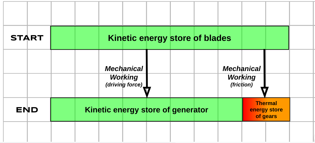
As an example, let’s consider a wind turbine used to generate electricity. As a starting point, let’s think about how much of the kinetic energy ‘harvested’ by the blades is transferred to the generator. The answer is, of course. not as much as we would hope. The majority is, hopefully, but a significant proportion is unavoidably lost via work done by friction to the thermal energy store of the gears.
This can be shown in a visually impactful way using the Bar Model approach:
Note that in this style of energy transfer diagram, the Principle of Conservation of Energy is communicated visually via the width of the bars. The bottom ‘End’ bar has to be exactly the same width as the top ‘Start’ bar.
What happens if a helpful maintenance engineer tops up the oil reservoir of the wind turbine? Well, we have a much happier situation, as shown below.
As we can see, a much greater proportion of the total energy is transferred usefully (and can be used to generate electrical power) in a well-maintained wind turbine.
Using energy efficient appliances in the home
How can we explain the advantages of using more efficient appliances in the home?
A diagram like this can help. The household that uses less efficient appliances has to buy more energy from their energy supplier to achieve exactly the same outcomes as the first. This is both more costly for the household as well as demanding that more resources are needed to generate electricity for no good reason.
Parachute vs. no parachute
Exactly the same amount of energy is transferred from the gravitational energy store of a parachutist whether their parachute deploys successfully or not. However, in the case of a successful deployment, much more energy is transferred into the thermal energy store of the surroundings than into their kinetic energy store. This helps ensure a safe landing!
I think that teaching vectors to 14-16 year olds is a bit like teaching them to play the flute; that is to say, it’s a bit like teaching them to play the flute as presented by Monty Python (!)
Part of the trouble is that the definition of a vector is so deceptively and seductively easy: a vector is a quantity that has both magnitude and direction.
There — how difficult can the rest of it be? Sadly, there’s a good deal more to vectors than that, just as there’s much more to playing the flute than ‘moving your fingers up and down the outside'(!)
What follows is a suggested outline teaching schema, with some selected resources.
Resultant vector = total vector: the ‘I’ phase
‘2 + 2 = 4’ is often touted as a statement that is always obviously and self-evidently true. And so it is — arithmetically and for mere scalar quantities. In fact, it would be more precisely rendered as ‘scalar 2 + scalar 2 = scalar 4’.
However, for vector quantities, things are a wee bit different. For vectors, it is better to say that ‘vector 2 + vector 2 = a vector quantity with a magnitude somewhere between 0 and 4’.
For example, if you take two steps north and then a further two steps north then you end up four steps away from where you started. Also, if you take two steps north and then two steps south, then you end up . . . zero steps from where you started.
So much for the ‘zero’ and ‘four’ magnitudes. But where do the ‘inbetween’ values come from?
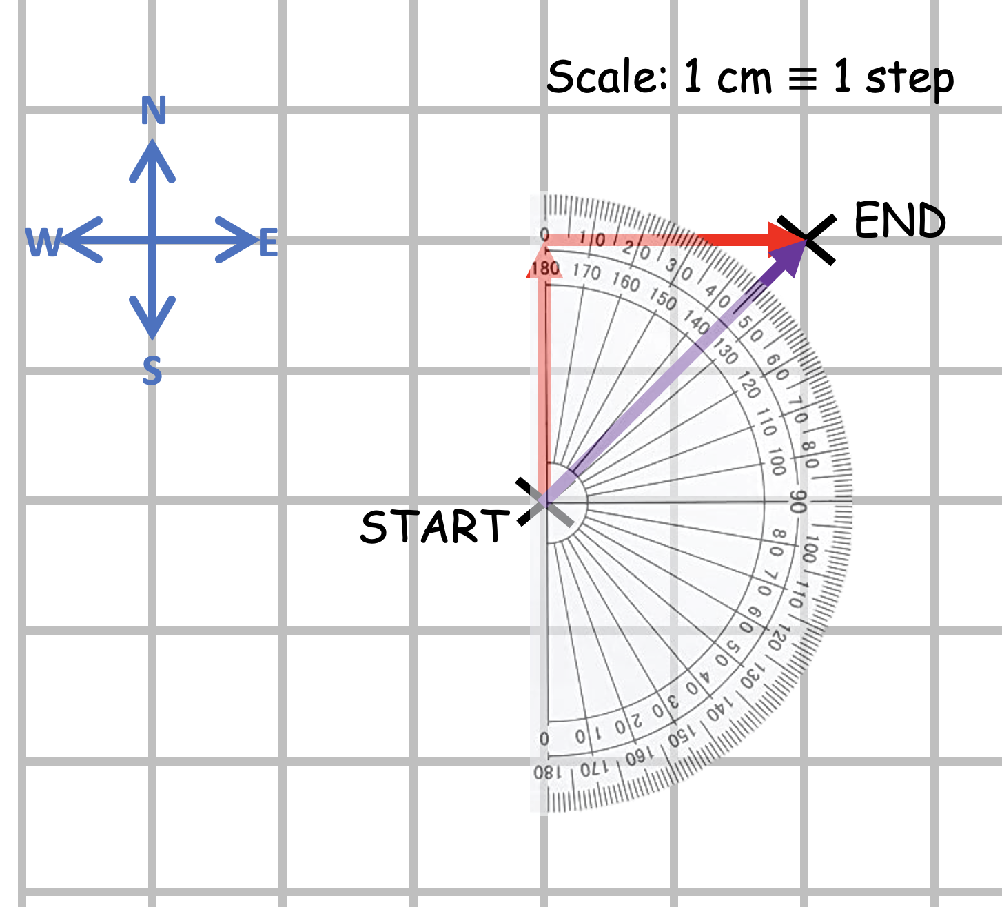
Simples! Imagine taking two steps north and then two steps east — where would you end up? In other words, what distance and (since we’re talking about vectors) in what direction would you be from your starting point?
This is most easily answered using a scale diagram.
To calculate the vector distance (aka displacement) we draw a line from the Start to the End and measure its length.
The length of the line is 2.8 cm which means that if we walk 2 steps north and 2 steps east then we up a total vector distance of 2.8 steps away from the Start.
But what about direction? Because we are dealing with vector quantities, direction just as important as magnitude. We draw an arrowhead on the purple line to emphasise this.
Students may guess that the direction of the purple ‘resultant’ vector (that is to say, it is the result of adding two vectors) is precisely north-east, but this can be a vague description so let’s use a protractor so that we can find the compass bearing.
And thus we find that the total resultant vector — the result of adding 2 steps north and 2 steps east — is a displacement of 2.8 steps on a compass bearing of 045 degrees.
Resultant vector = total vector: the ‘We’ phase
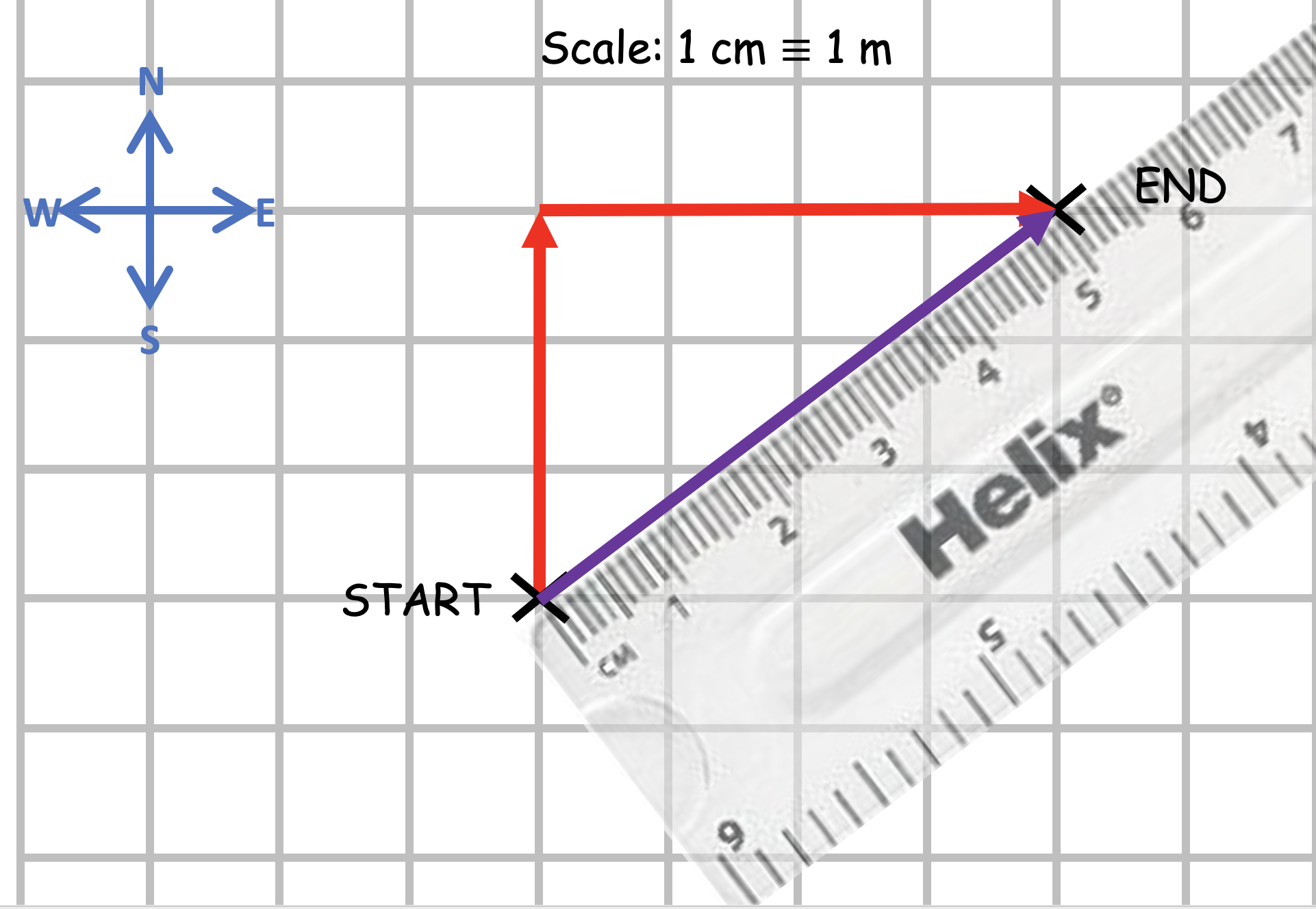
How would we go about finding the resultant vector if we moved 3 metres north and 4 metres east? If you have access to an interactive whiteboard, you could choose to use this Jamboard for this phase. (One minor inconvenience: you would have to draw the straight lines freehand but you can use the moveable and rotatable ruler and protractor to make measurements ‘live’ with your class.)
We go through a process similar to the one outlined above.
What would be a suitable scale?
How long should the vertical arrow be?
How long should the horizontal arrow be?
Where should we place the ‘End’ point?
How do we draw the ‘resultant’ vector?
What do we mean by ‘resultant vector’?
How should we show the direction of the resultant vector?
How do we find its length?
How do we convert the length of the arrow on the scale diagram into the magnitude of the displacement in real life?
The resultant vector is, of course, 5.0 m at a compass bearing of 053 degrees.
Resultant vector = total vector: the ‘You’ phase
Students can complete the questions on the worksheets which can be printed from the PowerPoint below.