Modelling Electrical Power Equations using the CTM

The Coulomb Train Model (CTM) is a straightforward, easily pictured representation that helps novice learners develop an initial “sense of mechanism” about how electric circuits work. You can read about it here and here (and, to some extent, track its development over time).

In this post, however, I want to focus on how effective the CTM is in helping students understand the energy and power formulas associated with electric circuits: notably E = QV, P = IV and P=I2R.

E=QV and the CTM

An animated version of the Coulomb Train Model

The E in E=QV stands for the energy transferred to the bulb by the electric current (in joules, J). The Q is the charge flow in coulombs, C. The V is the potential difference across the resistor in volts, V.

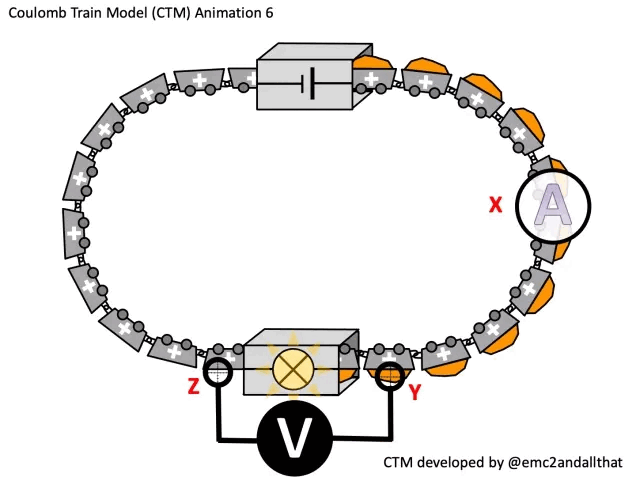
Using the Coulomb Train Model:

  • Each grey truck passing through the bulb represents one coulomb of charge flow. Q is therefore the number of grey trucks passing through the bulb in a certain time t. (We won’t specify what that time t is now but we will return to it shortly.)
  • The potential difference V is the energy transferred out of each coulomb as they pass through the bulb. If one joule (represented by the orange stuff in the truck) is transferred from each coulomb then the potential difference is one volt. If two joules then the potential difference is two volts, and so on.

How can we increase the energy transferred into the bulb? There are two ways:

  1. Increase the total number of coulombs passing through the bulb. That is to say, increasing Q. We could do this by (a) waiting a longer time so that more coulombs pass through the bulb; or (b) increasing the current so that more coulombs pass through each second.
  2. Increase the energy transferred from each coulomb into the bulb. That is to say, increasing V. We could do this by increasing the potential difference of the cell so that each coulomb is loaded up with more energy.
Hewitt representation of changing the values of Q and V while keeping the other fixed

Or, of course, we could increase the values of Q and V simultaneously.

Hewitt representation of increasing Q and V simultaneously

All you need is E = Q V

In other words, the energy transferred per second (or the power P in watts, W) is equal to the product of the current I in amperes (or coulombs per second) and the potential difference V in volts, V.

A higher current will increase the power transferred to the bulb: more coulombs will pass through the bulb per second so more energy is transferred to the bulb each second. This can be modelled using the Coulomb Train Model as shown:

Using the CTM to show the relationship between current I and power P

Increasing the potential difference V (i.e. the energy carried by each coulomb) would also increase P.

Deriving P=I2R from P=IV

If we start with P=IV but remember that V=IR then P=I(IR) so P=I2R.

This can be represented on the Coulomb Train Model like this:

We can increase the power transferred to the resistor by:

  • Increasing the value of the resistor (and keeping I constant, which implies that V would have to be increased). Doubling the value of R would double the value of P.
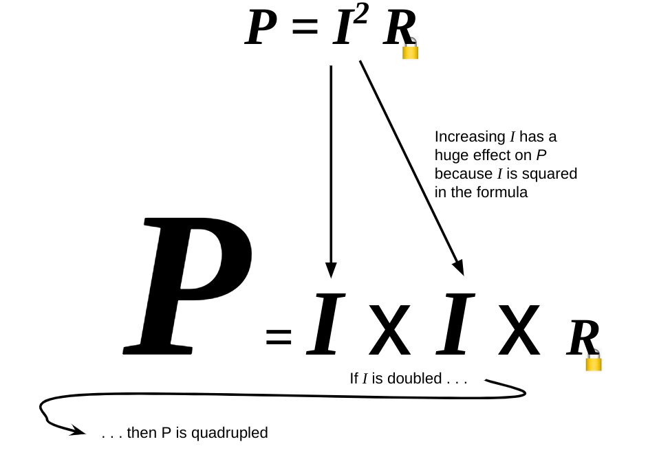
  • Increasing the value of I. However, since the formula includes I squared then this would have a disproportionate effect on P. For example, if I was doubled then P would be quadrupled. A Hewitt representation can be useful for highlighting this to students; for example:
A Hewitt representation of the effect of doubling I on P

Linking the electrical power formulas

The electrical power equations when considered in isolation can seem random and unconnected. Making the links between them explicit can be not just a powerful aid to memory, but also hints at the power and coherence of that noble exploration of reality and possibility called physics.

The Coulomb Train Model Revisited (Part 3)

In this post, we will look at explaining electrical resistance using the Coulomb Train Model.

This is part 3 of a continuing series (click to read part 1 and part 2).

The Coulomb Train Model (CTM) is a helpful model for both explaining and predicting the behaviour of real electric circuits which I think is useful for KS3 and KS4 students.

Without further ado, here is a a summary.

A summary of the Coulomb Train Model

Representing Resistance on the CTM

To measure resistance, we would set up this circuit.

We can represent this same circuit on the CTM as follows:

If we count how many ‘coulombs’ (grey trucks) pass one point in a certain time then on this animation we get 5 coulombs in 20 seconds.
This is equivalent to a current of
5 coulombs / 20 seconds = 0.2 coulombs per second = 0.2 amperes.

This way of thinking about current is consistent with the formula charge flow = current x time or Q=It which can be rearranged to give I=Q/t.

We have used identical labels on the circuit diagram and the CTM animation to encourage students to view them as different representations of a real situation. The ammeter at X would read 0.2 amps. We could place the ammeter at any other point in the circuit and still get a reading of 0.2 amps since ammeters only ‘count coulombs per second’ and don’t make any measurement of energy (represented by the orange substance in the trucks).

However, the voltmeter does make a measurement of energy: it compares the energy difference between a single coulomb at Y and a single coulomb at Z. If (say) 1.5 joules of energy is transferred from each coulomb as it passes through the bulb from Y to Z then the voltmeter will read a potential difference (or ‘voltage’ if you prefer) of 1.5 volts.

This way of thinking about potential difference is consistent with the formula energy transferred = charge flow x potential difference or E=QV which we can rearrange to give V=E/Q.

So as you can see, one volt is really equivalent to an energy change of one joule for every coulomb (!)

We can calculate the resistance of the bulb by using R=V/I so R = 1.5/0.2 = 7.5 ohms.


Resistance is not futile . . .

Students sometimes have difficulty accepting the idea of a ‘resistor’: ‘Why would anyone in their right minds deliberately design something that reduces the flow of electric current?’ It’s important to explain that it is vital to be able to control the flow of electric current and that one of the most common electronic components in your phone or games console is — the humble resistor.

One of many resistors on a circuit board. The colour codes tell us the value of each resistor.

Teachers often default to explaining electric circuits using bulbs as the active component. There is a lot to recommend this practice, not least the fact that changes in the circuit instantaneously affect the brightness of the bulb. However, it vital (especially at GCSE) to allow students to learn about circuits featuring resistors and other components rather than just the pedagogically overused (imho) filament lamp.


Calculating the resistance of a resistor

Consider this circuit where we have a resistor R1.

This can be represented as a coulomb train model like this:

The resistor does not glow with visible light as the bulb does, but it would glow pretty brightly if viewed through an infra red camera since the energy carried by the coulombs is transferred to the thermal energy store of the resistor. The only way we can observe this energy shift without such a special camera is to use a voltmeter.

Let’s begin by analysing this circuit qualitatively.

  • The coulombs are moving faster in this circuit than the previous circuit. This means that the current is larger. (Remember: current is coulombs per second.)
  • Because the current is larger, R1 must have a smaller resistance than the bulb. (Remember: resistance is a quantity that reduces the current.)
  • The energy transferred to each coulomb is the same in each example so the potential difference of the cell is the same in both circuits. (Of course, V can be altered by adding a second cell or turning up the setting on a power supply, but in many circuits V is, loosely speaking, a ‘fixed’ or ‘quasi-constant’ value.)
  • Because the ‘push’ or potential difference is the same size but the resistance of R1 is smaller, then the same cell is able to push a larger current around the circuit.

Now let’s analyse the circuit quantitatively.

  • 5 coulombs pass a single point in 13 seconds so the current is 5/13 = 0.38 coulombs per second = 0.4 amperes. (Double the current in the bulb circuit.)
  • The resistance can be calculated using R=V/I = 1.5/0.4 = 3.75 ohms. (Half the resistance of the bulb.)
  • Each coulomb is being loaded with 1.5 J of energy as it passes through the cell. Since this is happening twice as often in the resistor circuit as the bulb circuit, the cell will ‘go flat’ or ’empty its chemical energy store’ in half the time of the bulb cell.

So there we have it: more fun and high jinks with the CTM.

I hope that I have persuaded a few more teachers that the CTM is useful for getting students to think productively and, more importantly, quantitatively using correct scientific terminology about electric circuits.

In the next installment, we will look at series and parallel circuits.

The Coulomb Train Revisited (Part 2)

In this post, we will look at understanding potential difference (or voltage) using the Coulomb Train Model.

This is part 2 of a continuing series. You can read part 1 here.

The Coulomb Train Model (CTM) is a helpful model for both explaining and predicting the behaviour of real electric circuits which I think is suitable for use with KS3 and KS4 students (that’s 11-16 year olds for non-UK educators).

To summarise what has been discussed so far:


Modelling potential difference using the CTM

Potential difference is the ‘push’ needed to make electric charge move around a closed circuit. On the CTM, we can represent the ‘push’ as a gain in the energy of the coulomb. (This is consistent with the actual definition of the volt V = E/Q, where one volt is a change in energy of one joule per coulomb.)

How can we observe this gain in energy? Simple, we use a voltmeter.

Kudos to https://www.circuit-diagram.org/editor/ for the lovely circuit diagrams

On the CTM, this would look like this:

What the voltmeter does is compare the energy contained by two coulombs: one at A and the other at B. The coulombs at B, having passed through the 1.5 V cell, each have 1.5 joules of energy more than than the coulombs at A. This means that the voltmeter in this position reads 1.5 volts. We would say that the potential difference across the cell is 1.5 V. (Try and avoid talking about the potential difference ‘through’ or ‘of’ any part of the circuit.)


More potential difference measurements using the CTM

Let’s move the voltmeter to a different position.

On the CTM, this would look like this:

Let’s make the very reasonable assumption that the connecting wires have zero resistance. This would mean that the coulombs at C have 1.5 joules of energy and that the coulombs at D have 1.5 joules of energy. They have not lost any energy since they have not passed through any part of the circuit that actually has a resistance. The voltmeter would therefore read 0 volts since it cannot detect any energy difference.

Now let’s move the voltmeter one last time.

On the CTM, this would look like this:

Notice that the coulombs at F have 1.5 fewer joules than the coulombs at E. The coulombs transfer 1.5 joules of energy to the bulb because the bulb has a resistance.

Any part of the circuit that has non-zero resistance will ‘rob’ coulombs of their energy. On this very simple model, we assume that only the bulb has a resistance and so only the bulb will ‘push back’ against the movement of the coulombs and cost them energy.

Also on this simple model, the potential difference across the bulb is identical to the potential difference across the cell — but this is not always the case. For example, if the wires had a small but non-negligible resistance and if the cell had an internal resistance, but these would only come into play at A-level.

The bulb is shown as ‘flashing’ on the CTM to provide a visual cue to help students mentally model the transfer of energy from the coulombs to the bulb. In reality, instead of just one coulomb transferring a largish ‘chunk’ of energy, there would be approximately 1.25 billion billion electrons continuously transferring a tiny fraction of this energy over the course of one second (assuming a d.c. current of 0.2 amps) so we wouldn’t see the bulb ‘flash’ in reality.


How do the coulombs ‘know’ how much energy to drop off?

This section is probably more of interest to specialist physics teachers, but all are welcome.

One frequent criticism of donation models like the CTM is how do the coulombs ‘know’ to drop off all their energy at the bulb?

The response to this, of course, is that they don’t. This criticism is an artefact of an (arguably) over-simplified model whereby we assume that only the bulb has resistance. The energy carried by the coulombs according to this model could be shown as a sketch graph, and let’s be honest it does look a little dodgy…

But, more accurately, of course, the energy loss is a process rather than an event. And the connecting wires actually have a small resistance. This leads to this graph:

Realistically speaking, the coulombs don’t lose all their energy passing through the bulb: they merely lose most of their energy here due to the process of passing through a high resistance part of the circuit.

In part 3 of this series, we’ll look at how resistance can be modelled using the CTM.

You can read part 3 here.