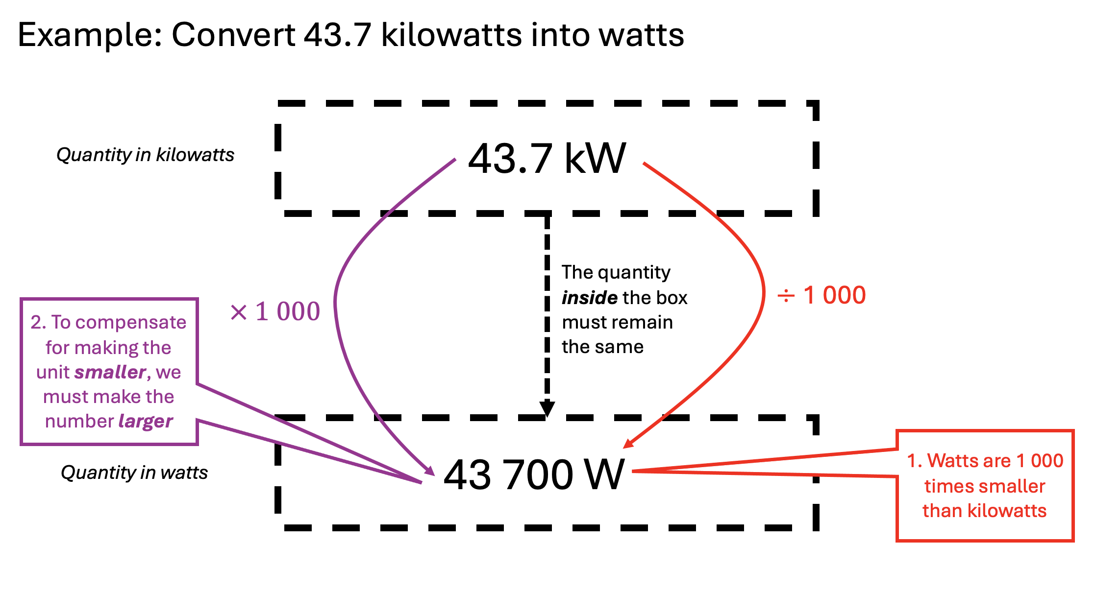
As I have written before, many students struggle with unit conversions. The Porter Method helps students’ understanding by making the process explicit.
Using the Porter Method to explain the mysteries of unit conversions
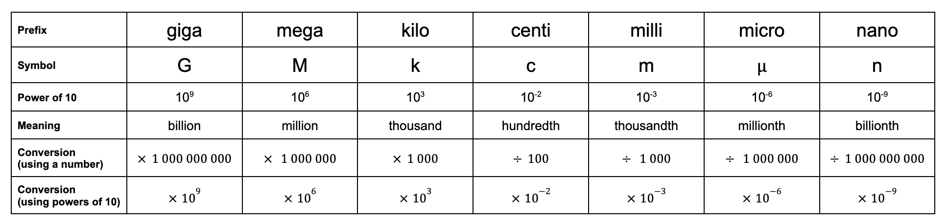
As of the time of writing, GCSE Science (2015 specification) students are expected to know the SI unit prefixes from giga- to nano-.
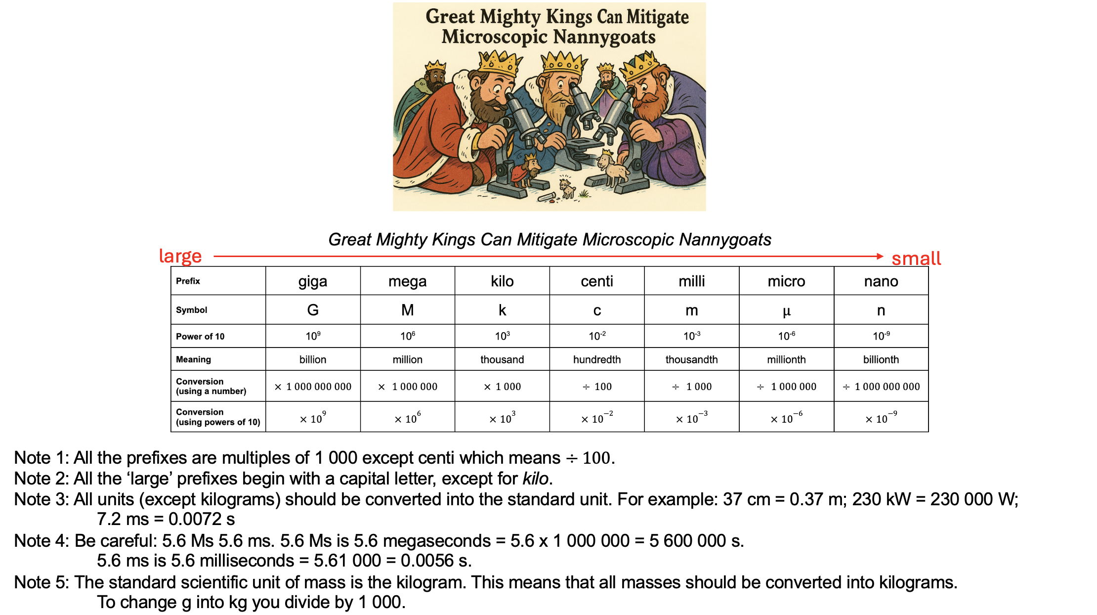
I suggest the following mnemonic:
A mnemonic for memorising the SI unit prefixes needed for GCSE
Choosing a mnemonic can be difficult because ‘mega’, ‘milli’ and ‘micro’ all begin with m, and even the first two letters of ‘milli’ and ‘micro’ are both ‘mi’. The mnemonic about helps students remember the difference between ‘milli’ and ‘micro’ by using ‘microscopic’ to help.
If you think this approach will be useful for your students, the Powerpoint is attached.
Enjoy!
PS You can find more of my thoughts on the SI system here
D. J. Griffiths’ (2013) genius re-statement of Lenz’s Law, modelled on Aristotle’s historically influential but now debunked aphorism that ‘Nature abhors a vacuum’
A student recently asked for help with this AQA A-level Physics multiple choice question:
AQA A-level Physics question from 2019 Paper 2
This question is, of course, about Lenz’s Law of Electromagnetic Induction. The law can be stated easily enough: ‘An induced current will flow in a direction so that it opposes the change producing it.’ However, it can be hard for students to learn how to apply it.
What follows is my suggested explanatory sequence.
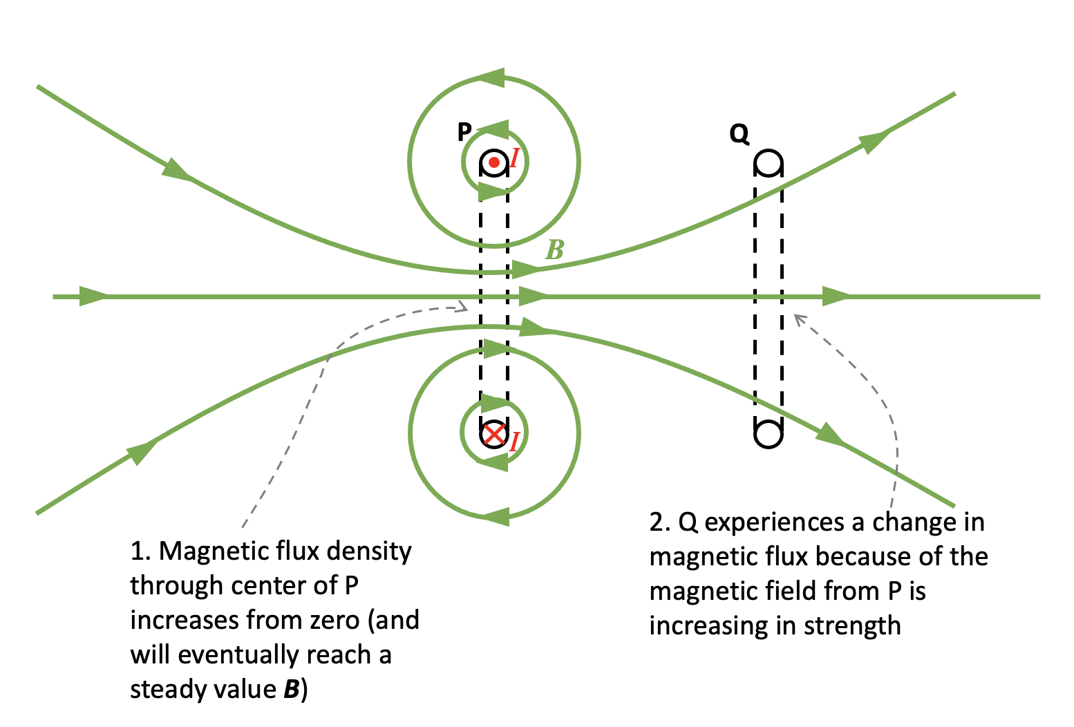
Step 1: simplify the diagram using the ‘dot and cross’ convention
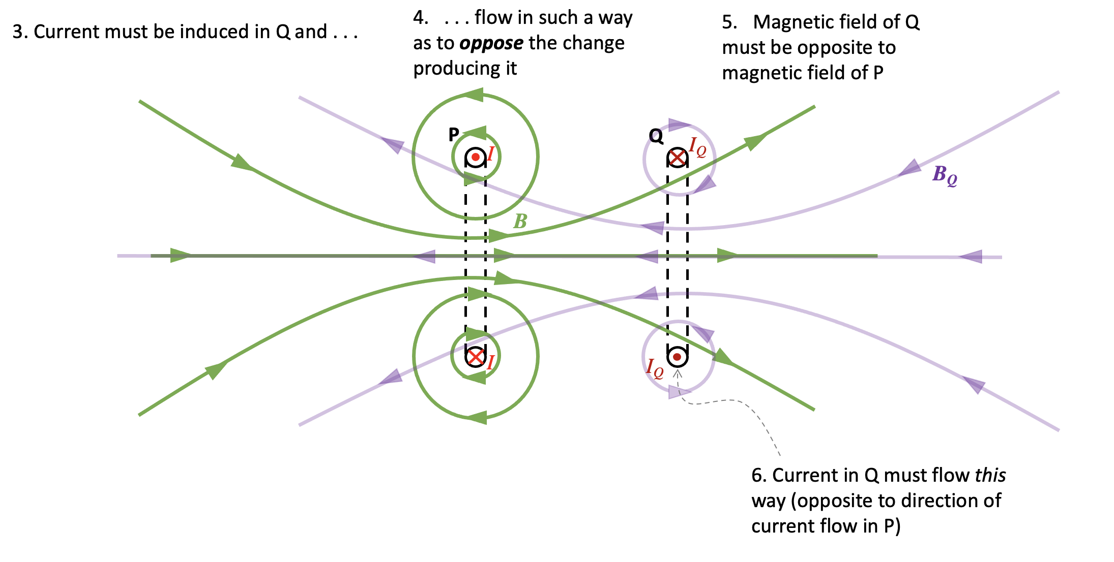
When the switch is closed, a current I begins to flow in coil P. We can assume that I starts at zero and increases to a maximum value in a very small but not negligible period of time.
Simplified 2D representation of the top diagram. The current directions I are arbitrary based on my ‘best guess’ interpretation of the 3D diagram and could be reversed if desired.
Step 2: consider the magnetic field produced by P
You can read more about a simple method of deducing the direction of the magnetic field produced by a coil or a solenoid here.
Step 3: apply Faraday’s Law to coil Q
Since Q is experiencing a change in magnetic flux, then an induced current will flow through it.
Step 4: apply Lenz’s Law to coil Q
The current in coil Q must flow in such a direction so that it opposes the change producing it.
Since P is producing an increasing magnetic flux through Q, then the current in Q must flow in such a way so that it tries to prevent the increase in magnetic flux which is inducing it. The direction of the magnetic field BQ produced by Q must therefore be opposite to the direction of the magnetic field produced by P.
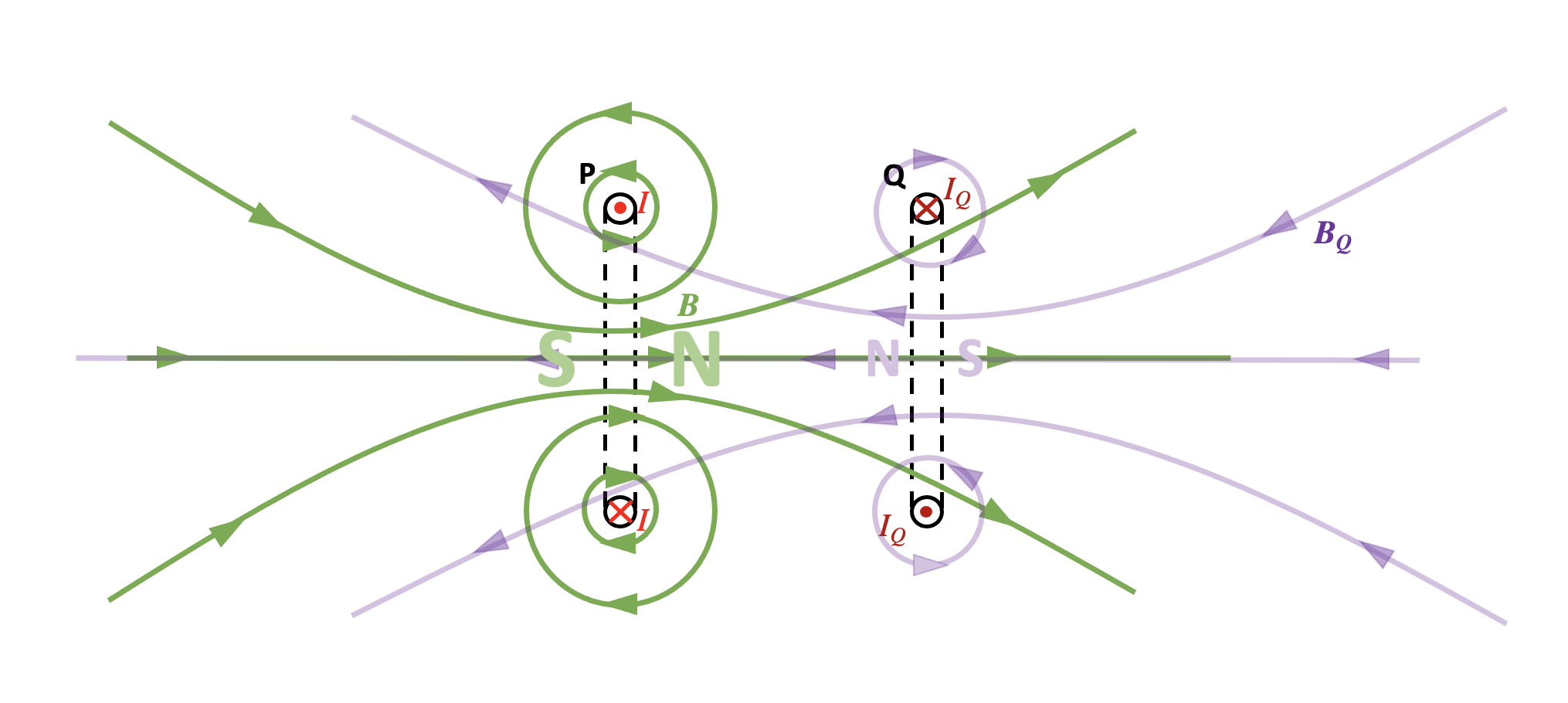
Step 5: consider the polarity of the magnetic fields of P and Q
We can see the magnetic field lines of coil P produce a north magnetic field on its right hand side. The magnetic field of Q will produce a north magnetic field on its left hand side. Coil P will therefore push coil Q to the right.
It follows that we can eliminate options A and C from the question.
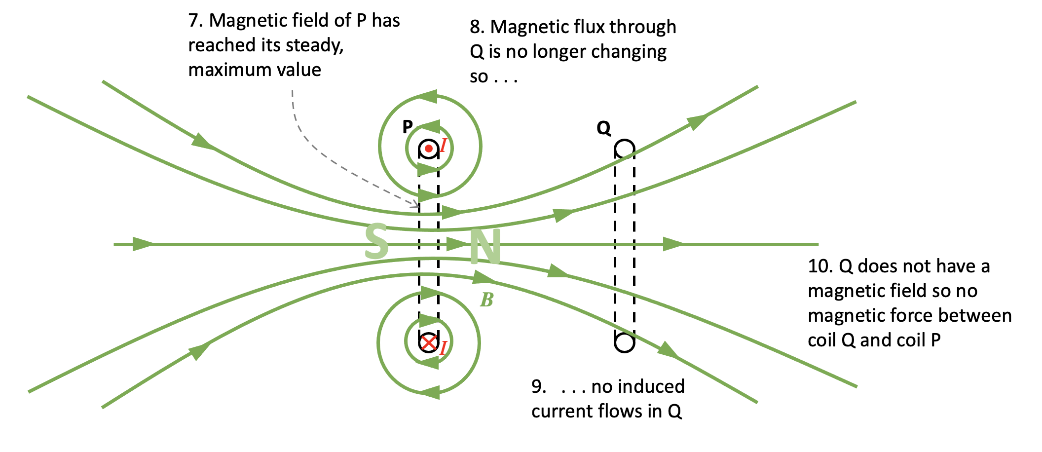
Step 6: What happens when the magnetic field of P reaches its steady value?
Because the magnetic field produced by coil P has how reached its steady maximum value, this means that the magnetic flux through coil Q also has a constant, unchanging value. Since there is no change in magnetic flux, then this means that no emf is induced across the coil so no induced current flows. Since Q does not have a magnetic field it follows that there is no magnetic interaction between them.
The answer to the question must therefore be D.
Step 7: check student understanding
For the alternative question, the correct answer of C can be explained by going through a process similar to the one outlined above.
When the switch is opened, the magnetic flux through Y begins to decrease.
A changing magnetic flux through Y induces current flow.
Lenz’s Law predicts that the direction of this current is such that it opposes the change producing it.
The current through Y will therefore be in the same direction as the current through X to produce a magnetic field in the same direction.
The coils will attract each other.
Eventually, the magnetic flux produced by coil X drops to a constant value of zero.
Since there is no change in magnetic flux through Y, there is no induced current flow through Y and hence no magnetic field.
There is no magnetic interaction between X and Y and therefore the force on Y is zero.
Conclusion
I hope teachers find this detailed analysis of a Lenz’s Law question useful! As in much of A-level Physics, the devil is not in the detail but rather in the application of the detail. Students who encounter more examples will have a more secure understanding.
Reference
Griffiths, David (2013). Introduction to Electrodynamics. p. 315.
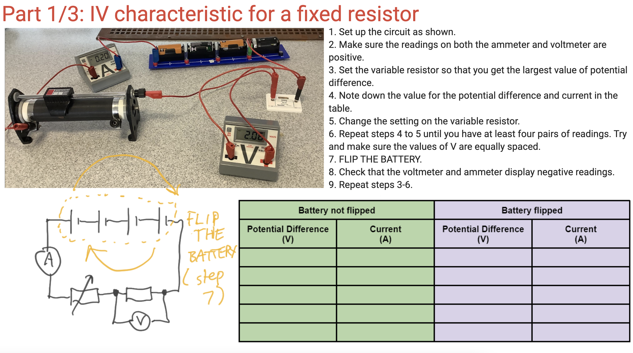
What is the worst circuit in the world? Many teachers think it is the one below.
This is the circuit that AQA (2018: 47) strongly suggest should be used to capture the data for plotting IV characteristics (aka current against potential difference graphs) for a fixed resistor, a filament lamp and a diode. The reasons why it is ‘the worst circuit in world’ were outlined in part one; and also some reasons why, nonetheless, schools teaching the 2016 AQA GCSE Physics / Combined Science specifications should (arguably) continue to use it.
The procedure outlined isn’t ‘perfect’ but works well using the equipment we have available and enables students to capture (and plot using a FREE Excel spreadsheet!) the data with only minor troubleshooting from the teacher.
Step the first: ‘These are the graphs you’re looking for.’
I find this required practical runs more smoothly if students have some awareness of what kind of graphs they are looking for. So, to borrow a phrase, I usually just tell ’em.
You can access an unannotated version of the slides on Google Jamboard and pdf below.
Step the second: capture the data for the fixed resistor
It is a continual source of amazement to me that students seem to find a photograph of a circuit easier to interpret than a nice, clean, minimalist circuit diagram, so for an easier life I present both.
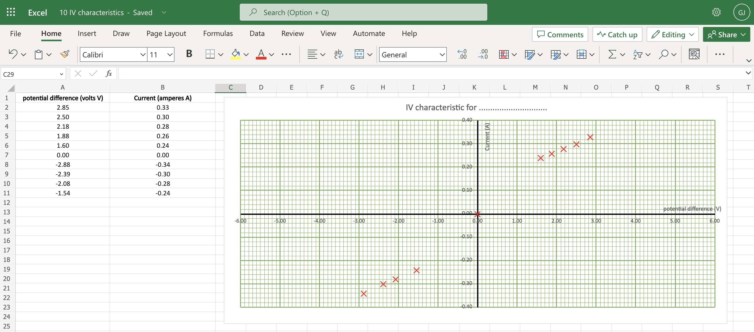
You can, if you have access to ICT, get the students to plot their results ‘live’ on an Excel spreadsheet (link below). I think this is excellent for helping to manage the cognitive demand on our students (as I have argued before here). Please note that I have not used the automated ‘line of best fit’ tools available on Excel as I think it is important for students to practice drawing lines of best fit — including, especially, curved lines of best fit (sorry, Maths teachers, in science there are such things as curved lines!)
Results for a fixed resistor from a typical group of students. These results are clearly consistent with a straight line of best fit going through the origin. However, they can be criticised for not being evenly spaced across the range — but this is a limitation of using the ‘worst circuit in the world’ and, happily(!), gives the students something to write about in their evaluation.
Step the second: capture the data for the filament lamp
In this circuit, we replaced the previous 0-16 ohm variable resistor with a 0 – 1000 ohm variable resistor paired with 2.5 V, 0.2 A filament lamp because the bulb has a resistance of about 60 ohms when run at 2.5 V and so the 0-16 ohm variable resistor is often ineffective. We allowed a maximum potential difference of just over 3.0 V to ‘over run’ the bulb so as to be sure of obtaining the ‘flattening’ of the graph. The method calls for very small adjustments of the variable resistor to obtain noticeable changes of brightness of the bulb. Note that the cells used in the photograph had seen many years of service with our physics department(!) and so were fairly depleted such that three of them were needed to produce a measly three volts; you would likely only need two ‘fresher’, ‘newer’ cells to achieve the same.
These are the results obtained by a typical student group. The results are clearly consistent with the elongated ‘S’ shaped curve predicted from theory. The results can be criticised for clustering, but this can be addressed by students in their evaluation of the experiment.
Step the third (sub-parts a and b): capturing the data for a diode
Results for diode captured by a group of students following the procedure outlined above.
And, by popular request, a copy of the PowerPoint below (although, trust me, I think Google Jamboard is superior when using ‘live’ in front of a class)
“The most miserable latch that’s ever been designed in the history of mankind or before.”
Astronaut Jack R. Lousma commenting on some equipment issues during the NASA Skylab 3 mission (July to September 1973), quoted in Cooper 1976: 41
What does the worst circuit that’s ever been designed in the history of humankind or before look like? Without further ado, here it is:
‘But wait,’ I hear you say, ‘isn’t this the circuit intended for obtaining the data for plotting current-potential difference characteristic curves as recommended by the AQA exam board in their GCSE Physics and GCSE Combined Science specifications?’ (AQA 2018: 47)
Sadly, it is indeed.
Why is ‘the standard test circuit’ a *bad* circuit?
The point of this required practical is to get several paired readings of potential difference across a component and the current through a component to enable us to plot a graph (aka ‘characteristic’) of current against potential difference. Ideally, we would like to start at 0.0 volts across the resistor and measure the current at (say) 1.0, 2.0, 3.0, 4.0, 5.0 and 6.0 volts. That is to say, we would like to treat the potential difference as the independent variable and adjust it in consistent, regular increments.
Now let’s say we use a typical school rheostat such as the one shown below as the variable resistor in series with the 10 ohm resistor. The two of them will behave as a potential divider circuit (see here and here for posts on this topic).
The resistance of the variable resistor can be varied between 0 and 16 ohms by moving the slider. When the slider is at A it will have the maximum resistance of 16 ohms and zero when it is at C, and in-between values at any other point.
A typical school rheostat. To use as a simple variable resistor, connect only terminals A and C into the circuit. (Please note: using terminals B and C will make it behave as a fixed resistor.)
When the slider is at C, the 10 ohm resistor gets the full potential difference from the supply and so the voltmeter will read 6.0 V and the ammeter will read (using I=V/R) 6.0 / 10 = 0.6 amps.
When the slider is at A, the total resistance of the circuit is 10 + 16 = 26 ohms so the ammeter reading (again using I=V/R) will be 6.0/26 = 0.23 amps. This means that the voltmeter reading (using V=IR) will be 0.23 x 10 = 2.3 volts.
This means that the circuit as presented will only allow us to obtain potential differences between a minimum of 2.3 V and a maximum of 6.0 V across the component by moving the slider between B and C, which is less than ideal.
‘It is a far, far better circuit that I build than I have ever built before…’
It is a far, far better thing that I do, than I have ever done.
Charles Dickens, ‘A Tale of Two Cities’
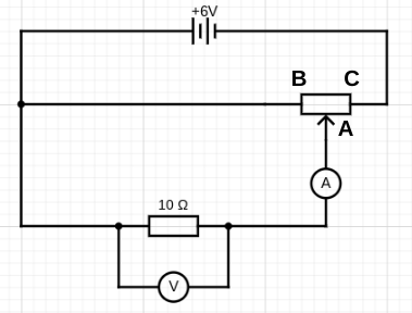
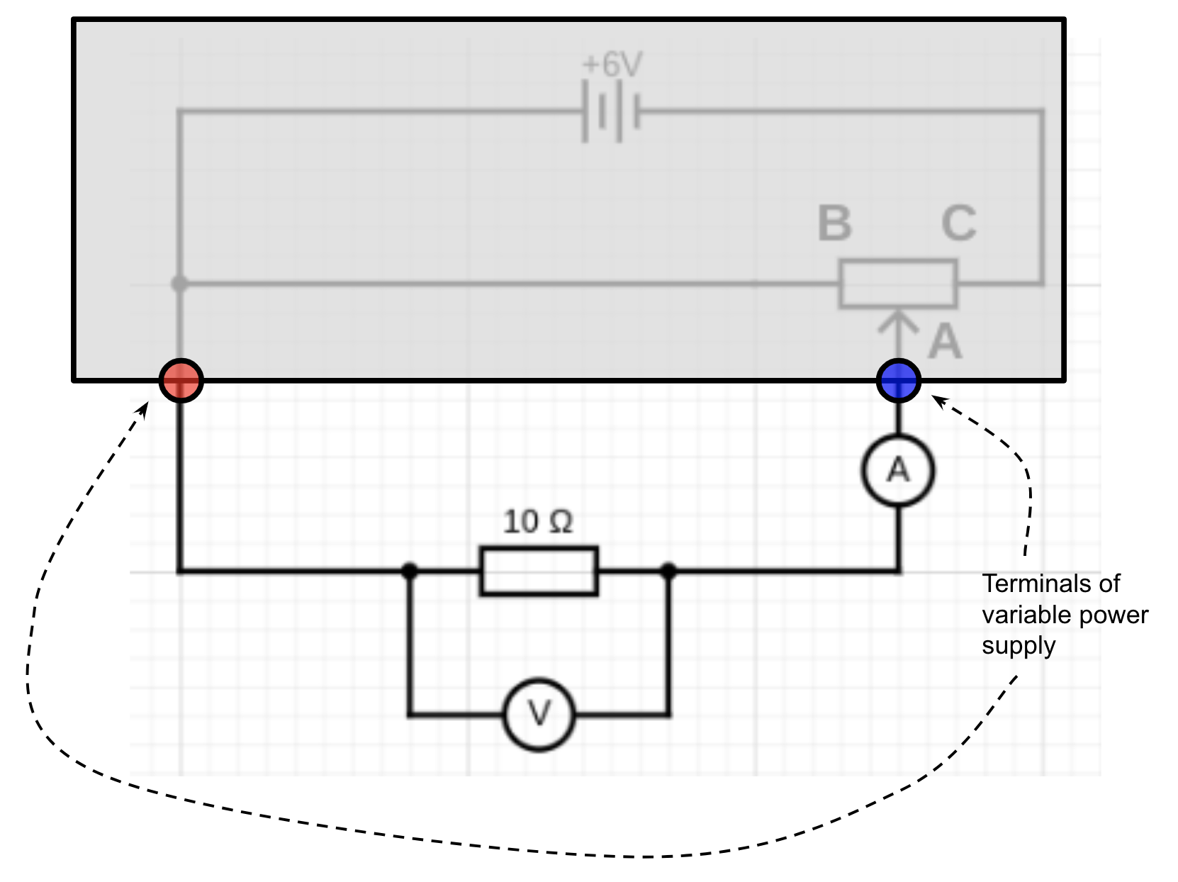
This circuit is a far better one for obtaining the data for a current-potential difference graph. This is because we can access the full 0.0 V to 6.0 V of the supply simply by adjusting the position of the rheostat slider. The rheostat is being used as a potential divider in this circuit rather than as a simple variable resistor.
When the slider is at B, the voltmeter will read 0.0 V and the current through the 10 ohm resistor will be 0.0 amps. A small movement of the slider from B towards C will increase the reading of the voltmeter to (say) 1.0 V and the ammeter would read 0.1 A. Further small movements of the slider will gradually increase the potential difference across the resistor until it reaches the full 6.0 V when the slider is at C.
A-level Physics students are expected to be able to use this circuit and enumerate its advantages over the ‘worst circuit in the world’.
And, to be fair, AQA do suggest a workaround that will allow GCSE student to side-step using ‘the worst circuit in the world’:
If a lab pack is used for the power supply this can remove the need for the rheostat as the potential difference can be varied directly. The voltage should not be allowed to get so high as to damage the components, check the rating of the components you plan to suggest your students use.
AQA 2018: 16
A ‘lab pack’ i.e. a power supply with a variable output potential difference
If this method is used, then in effect you would be using the ‘built in’ rheostat inside the power supply.
So why not use the superior potential divider circuit at GCSE?
The arguments in favour of using ‘the worst circuit in the world’ as opposed to the more fit for purpose potential divider circuit are:
The ‘worst circuit in the world’ is (arguably) conceptually easier than the potential divider circuit, especially if students have not studied series and parallel circuit before. This allows more freedom in sequencing when IV characteristics are taught.
A fuller range of potential differences can be accessed even using the ‘worst circuit in the world’ if the maximum value of the variable resistor is much larger than the resistance of the component. For example, if we used a 0 – 1 kilo-ohm variable resistor in series with the 10 ohm resistor then very fine adjustments of the variable resistor would allow a suitable range of potential difference to be applied across the component.
Students are often asked direct questions about the ‘worst circuit in world’.
Question from AQA Paper 1 (2021) where students who have used ‘the worst circuit in the world’ for their investigation would (imo) have an advantage over those that have not.
In the next post, I will outline how I introduce and teach this required practical — using, to my shame, ‘the worst circuit in the world’ — and also supply some useful resources.
Charged particles which are stationary within a magnetic field do not experience a magnetic force; however, charged particles which are moving within a magnetic field most definitely do. And, what is more, this magnetic force or Lorentz force always makes them move on circular paths or semicircular paths. (Note: for simplicity we’re only going to look at particles whose velocity is perpendicular to the magnetic field lines in this post.) The direction of the Lorentz force can be predicted using Fleming’s Left Hand Rule.
An understanding of this type of interaction is essential for A-level Physics as far the physics of particle accelerators and cyclotrons are concerned. It is, of course, desirable to be able to demonstrate this to our students in the school laboratory. Your school may be lucky enough to own an electron beam tube and a pair of Helmholtz coils that is the usual way of displaying this phenomenon.
Bob Worley (@UncleBo80053383) recently made me aware of a low cost, microscale chemistry demonstration that I believe shows this phenomenon to good effect. If the electrolysis of sodium sulfate is carried out over a strong neodymium magnet then the interaction between the electric and magnetic fields creates clear patterns of circulation that are consistent with the directions predicted by the movement of the ions within the electric field produced by the electrodes and the Fleming’s Left Hand Rule force on the ions produced by the external magnetic field.
Please note that in the following post, any errors, omissions or misconceptions are my own (especially with the chemistry ‘bits’).
Why do charged particles move on circular paths when they travel through magnetic fields?
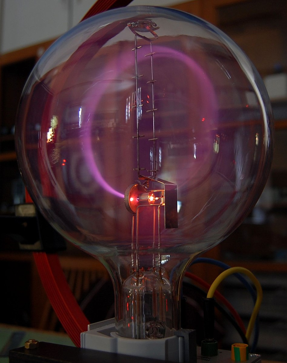
An electron beam tube. The electron beam is being made to move on a circular path by an external magnetic field.
In the diagram below, the green area represents a region of uniform magnetic flux density B. The field lines are directed into the plane of the diagram. Let’s consider an electron (1) fired at a horizontal velocity v from an electron gun as shown.
Fleming’s Left Hand Rule predicts that an upward force F will be produced on the electron. (Remember that the current in FLHR is conventional current so the ‘I’ finger should be pointed in the opposite direction to v because electron have a negative charge!) This will alter the direction of v so that the electron moves to position (2). Note that the magnitude of v is unaltered since F is acting at right angle to it. In position (2), FLHR again predicts a force F will act on the moving electron, and this force will again be at right angles to v resulting in the electron moving to position (3). Since the magnitude of v remains unaltered and F is always perpendicular to it, this means that F acts as a centripetal force which means that the electron travels at uniform speed around a circular orbit of radius r.
It can be shown that r = mv/Bq where m is the mass of the particle and q is its charge.
Setting up the electrolysis of sodium sulfate in a magnetic field
Electrolysis of sodium sulfate influenced by a magnet (side view)
The equipment is set up as shown in the diagram above. This can be seen from 0:00 to 0:10 seconds on the video. The magnetic field produced by the magnet can be thought of as a uniform vertical field through the volume of the drop.
Next, a few drops of red litmus are added. Since the sodium sulfate solution is neutral, the red litmus does not change colour.
At 0:15 seconds, the electrodes are introduced to the solution. Note that the anode is on the left and the cathode is on the right.
Observing the circular motion of charged particles in a magnetic field (part 1)
Almost immediately, we see indicator change colour next to the cathode. Since sodium sulfate is a salt produced using a reactive metal and an acid containing oxygen, the electrolysis will result in hydrogen gas at the cathode and oxygen at the anode. In other words, water will be electrolysed.
At the cathode, water molecules will be reduced to form H2 and OH–.
It is the OH– ions that produce the colour change to purple.
From 0:23 to 0:27 we can clearly an anticlockwise circulation pattern in the purple coloured region.
This can be explained by considering the forces on an OH– ion as shown on the diagram below.
Electrolysis of sodium sulfate under the influence of a magnetic field (plan view)
As soon as it is created, the OH– ion will be repelled away from the cathode along an electric field line (blue dotted lines). This means that it will be moving at a velocity v at the instant shown. However, due to the external magnetic field B it will also be subject to a Lorentz force F as shown (and whose direction can be predicted using Fleming’s Left Hand Rule) which will make it move on an anticlockwise circular path.
Because of the action of the electric field, the magnitude of v will increase meaning that that radius of circulation r of the OH– ion will increase. This means that OH– ion will travel on an anticlockwise spiral path of gradually increasing radius, as observed. This is analogous to paths followed by charged particles in a cyclotron.
Observing the circular motion of charged particles in a magnetic field (part 2)
At 0:29 seconds, we observe a second circulation pattern. We see the purple coloured solution begin a clockwise circulation around the anode.
This is because the OH– ions gradually move towards the anode and eventually will begin moving at a radial velocity v towards it as shown. Fleming’s Left Hand Rule predicts a Lorentz force F will act on the ion as shown which means that it will move on a clockwise circular path.
The video from 0:30 to 0:35 shows at least some the ions moving on clockwise spiral path of decreasing radius. This is most likely because the magnitude of v of a number of ions is decreasing. The mechanism which produces this decrease of v is unknown (at least to me) but it seems plausible to suppose that a large number of OH– ions arriving in the smaller region around the anode might produce a ‘traffic jam’ that would reduce the mean velocity of the ions here.
Conclusion
I hope physics teachers find this demonstration as useful and intriguing as I do. Please leave a comment if you decide to use it in your physics classroom. Many thanks to Bob Worley for posting the fascinating video!
However, the ancients still held fast to the idea that the Earth was the centre of the universe. This is often presented unfairly as a failure of intelligence or nerve on their part. However, they believed they had good evidence to support the idea. One of the more convincing arguments advanced in favour of geocentrism was the absence of stellar parallax. Surely, if the Earth described a vast circle around the Sun in one year, then we would observe some shift in the positions of the fixed stars? Just as we would observe the nearer trees shift against the background of the distant hills as we walked through the landscape. The absence of stellar parallax could only be explained by (a) the fixity of the Earth; or (b) the fixed stars were absurdly distant so stellar parallax was too small to be observed.
Robert Hooke’s attempt to measure stellar parallax
In 1674, Robert Hooke (1635-1703) attempted to measure stellar parallax and put an end to one of the more powerful arguments of the anti-Copernicans. He built a zenith telescope (that is to say, a telescope that only points vertically upwards) that extended through the roof of his house in order to observe Gamma Draconis, a star that can be seen directly overhead in London. He recorded a total of four observations and calculated its annual parallax as 30 seconds of arc, that is 30/3600ths of one degree. His contemporaries remained unconvinced, mostly because he had only made four observations.
Modern astronomers have measured the distance of Gamma Draconis to be 153.4 light years, giving it an annual parallax of 0.02 seconds of arc: Robert Hooke’s measurement was 1500 times the actual value, so it would appear that, although his methodology was sound, his instrumentation was not up to the task.
And so it would remain until the 1830s when telescope technology had improved to the point where stellar parallaxes could be accurately measured.
However, Scottish mathematician and astronomer James Gregory (1638-1675) had suggested and acted on an intriguing alternative in 1668.
James Gregory FRS (1638-1675)
Before discussing Gregory’s method, we will look at Christiaan Huygens (1629-1695) later, more famous but — as I shall argue — less accurate method for measuring the distance to Sirius.
Christiaan Huygens’ calculation of the distance to Sirius (1698)
Many astronomers had suggested that we could estimate the distance to the stars if:
we assume that the Sun is a typical star so that other stars have a similar size and luminosity;
we compare the brightness of the Sun to a given star; and
we use the inverse square law to calculate how much further away the star is than the Sun given their relative brightnesses.
The problem was: how can we reliably compare the brightness of the Sun and a given star?
Huygens tried to do this by observing the Sun through a small hole and making the hole smaller until it appeared to match his memory of the brightness of Sirius as observed previously.
Diagram showing Huygens’ method for comparing the luminosity of the Sun and the star Sirius
This is obviously a highly subjective method since Huygens was relying not only on his memory, but also on the memory of an observation made under very different observing conditions. Huygens did take steps to make the observing conditions as similar as possible: for example, he viewed both the Sun and Sirius through a long 4 metre tube to eliminate light from other sources. (Please be aware, that observing the Sun directly, even through a small aperture, is extremely dangerous!)
The difficulty was compounded by the fact that Huygens lacked the technology to make the hole in the brass plate small enough to mimic the appearance of Sirius; he improvised by adding a small microscope(!) lens to scatter the light but this, of course, added another layer of complication. Nonetheless, he was able to estimate the distance to Sirius as being 27664 times the Earth-Sun distance or 0.44 light-years. This is indeed in the right ball park. The modern distance is given as 8.6 light-years which is much further than Huygens’ measurement, partly because Sirius isn’t a star similar to the Sun: Sirius is actually 25.4 times brighter than our local star so is even more distant than Huygens supposed.
James Gregory’s method for calculating the distance to Sirius (1668)
Gregory suggested using a planet as an intermediary in comparing the brightness of the Sun to Sirius.
Diagram showing James Gregory’s method for comparing the luminosity of the Sun and the star Sirius
In 1668, in his ‘Geometriae pars universalis’, James Gregory set out a method for solving the challenging technical problem of actually determining the ratio of the apparent brightness of the Sun as compared with that of a bright star such as Sirius. He proposed using a planet as an intermediary between the Sun and Sirius. We are to observe the planet at a time when its brightness exactly equals that of Sirius, so that the problem then reduces to one of comparing the brightness of the Sun with that of the planet. But the planet’s brightness depends upon the light it receives from the Sun (and therefore upon the brightness of the Sun), and upon quantities such as the size and reflectivity of the planet and distances within the solar system (quantities which we suppose to be accurately known). A simple calculation then yields the required value. Gregory himself obtained [a value of] 83,190 [times the Earth-Sun distance], but he tells us that with more accurate information on the solar system the figure would be greater still
Hoskin (1977)
Gregory’s method is not so subjective as Huygens’ because we would be viewing Jupiter and Sirius under very similar observing conditions and also would not have to rely on our memory of our perception of Sirius’ brightness. His value of 83190 times the Earth-Sun distance equates to 1.32 light-years. However, had he known that Sirius was 25.4 times brighter than the Sun, he would have increased the calculated distance by a factor equal to the square root of 25.4 which would give a value of 6.6 light-years — not bad, considering the modern value is 8.6 light-years!
Also, bear in mind that Gregory had to assume that Jupiter reflected 100% of the sunlight that fell on it since he had no information about Jupiter’s albedo (the proportion of light reflected by Jupiter’s surface) and had only quite sketchy estimates of Jupiter’s diameter. As Gregory correctly surmised, his figure was a lower boundary estimate for the distance of Sirius, which was likely to increase as more information came to light.
Newton and Gregory’s Method
Sir Isaac Newton (1624-1727) possessed a copy of Gregory’s book (Hoskin 1977: 222) and gave a detailed description of the method in The System of The World which, however, was only published in 1728 after Newton’s death.
In consequence, James Gregory’s brilliant proposal of 1668, which so quickly led Newton to a correct understanding of the distances to the nearest stars, was effectively in limbo until the second quarter of the eighteenth century. In its stead, students of astronomy were introduced to the method of Christiaan Huygens, which was based on the same assumptions but used a much inferior technique for comparing the brightness of the Sun and a star.
Hoskin 1977
The brain is wider than the sky, For, put them side by side, The one the other will include With ease, and you beside.
Emily Dickinson, ‘The Brain’
Reference
Hoskin, M. (1977). The English Background to the Cosmology of Wright and Herschel. In: Yourgrau, W., Breck, A.D. (eds) Cosmology, History, and Theology. Springer, Boston, MA.
The philosopher John Stuart Mill (1806-1873) offers an intriguing system for classifying misconceptions (or ‘fallacies’ as he terms them) that could be useful for teachers in understanding many of the misconceptions and preconceptions that our students hold.
My own thoughts on this issue have been profoundly shaped by the ‘Resources Framework‘ as presented by authors such as Andrea di Sessa, David Hammer, Edward Redish and others. What follows is not a rejection of this approach but rather an exploration of whether Mill’s work offers some relevant insights. My thought is that it quite possibly might; after all, it has happened before . . .
The authors, however, did not use or refer to Mill’s system of logic in developing the programs or in formulating their theory of instruction. They didn’t discover parallels between their theory of instruction and Mill’s logic until after they had finished writing the bulk of ‘Theory of Instruction’. The discovery occurred when they were writing a chapter on theoretical issues. In their search for literature relevant to their philosophical orientation, they came across Mill’s work and were shocked to discover that they had independently identified all the major patterns that Mill had articulated. ‘Theory of Instruction’ (1982) even had parallel principles to the methods in ‘A System of Logic’ (1843)
Engelmann and Carnine 2013: Chapter 2
Mill’s system for classifying fallacies
In A System of Logic (1843), Mill argues that
Indifference to truth can not, in and by itself, produce erroneous belief; it operates by preventing the mind from collecting the proper evidences, or from applying to them the test of a legitimate and rigid induction; by which omission it is exposed unprotected to the influence of any species of apparent evidence which offers itself spontaneously, or which is elicited by that smaller quantity of trouble which the mind may be willing to take.
Mill 1843: Book V Chap 1
Mill is saying that we don’t believe false things because we want to, but because there are mechanisms preventing our minds from duly noting and weighing the myriad evidences from which we construct our beliefs about the world by the process of induction.
He suggests that there are five major classes of fallacies:
A priori fallacies;
Fallacies of observation;
Fallacies of generalisation;
Fallacies of ratiocination; and
Fallacies of confusion
Erroneous arguments do not admit of such a sharply cut division as valid arguments do. An argument fully stated, with all its steps distinctly set out, in language not susceptible of misunderstanding, must, if it be erroneous, be so in some one of these five modes unequivocally; or indeed of the first four, since the fifth, on such a supposition, would vanish. But it is not in the nature of bad reasoning to express itself thus unambiguously.
Mill 1843: Book V Chap 1
Mill is saying that invalid inferences, by their very nature, are ‘messier’ and harder to classify than correct inferences. However, they must all fit into the five categories outlined above. Actually, they are more likely to fit into the first four categories since clear and unambiguous use of language and terms would tend to eliminate fallacies of confusion as a matter of course.
What is an a priori fallacy?
In philosophy, a priori means knowledge derived from theoretical deduction rather than from empirical observation or experience.
Mill says that a priori fallacies (which he also calls fallacies of simple observation) are
those in which no actual inference takes place at all; the proposition (it cannot in such cases be called a conclusion) being embraced, not as proved, but as requiring no proof; as a self-evident truth.
Mill 1843: Book V Chap 3
In other words, an a priori fallacy is an idea whose truth is accepted on its face value alone; no evidence or justification of its truth is needed. An example from physics education might be ideas such as ‘heavy objects fall’ or ‘wood floats’. Some students accept these as obvious and self-evident truths: there is no need to consider ideas such as weight and resultant force or density and upthrust because these are ‘brute facts’ about the world that admit of no further explanation. This a case of mislabelling subjective facts as objective facts.
Falling is a location-specific behaviour: objects on Earth will indeed tend to accelerate downwards towards the centre of the Earth: this is a subjective fact which is dependent on the location of the object rather than an objective fact about the behaviour of all objects everywhere (although we could, of course, argue that falling is indeed an objective fact about objects which are subject to the influence of gravitational fields). Equally, floating is not a phenomenon restricted to the interaction between wood and water: many woods will sink in low density oils. ‘Wood floats‘ is not an objective fact about the universe but rather a subjective fact about the interaction of wood with a certain liquid.
This may be why some students are incurious about certain phenomena because they regard them as trivial and obvious rather than manifestations of the inner workings of the universe.
Mill lists many other examples of the a priori fallacy, but his examples are drawn from the history of science and philosophy, and so are of less direct relevance to the science classroom, with the possible exception of the two following examples:
Humans tend to default to the assumption that any phenomenon must necessarily have only a single cause; in other words, we assume that a multiplicity of causes is impossible. We are protected from this version of the a priori fallacy by the guard rail of the scientific method. For a complete understanding of a phenomenon, we look at the effect of one independent variable at a time whilst controlling other possible variables.
There remains one a priori fallacy or natural prejudice, the most deeply-rooted, perhaps, of all which we have enumerated; one which not only reigned supreme in the ancient world, but still possesses almost undisputed dominion over many of the most cultivated minds … This is, that the conditions of a phenomenon must, or at least probably will, resemble the phenomenon itself … the natural prejudice which led people to assimilate the action of bodies upon our senses, and through them upon our minds, to the transfer of a given form from one object to another by actual moulding.
Mill 1843: Book V Chap 3
I think that this tendency might be the one in play with the difficulties that many students have with understanding how images are formed: they think that an image is an evanescent ‘clone’ of the object that is being imaged rather than being an artefact of the light rays reflected or emitted from the object. This also might help explain why students find explaining the colour changes produced by looking at an object through a colour filter or illuminating it with coloured light difficult: they assume that colour is an essential unalterable property that adheres to the object and cannot be changed without changing the object.
We’ll continue this exploration of Mill’s classification of misconceptions in later posts.
References
Engelmann, S., & Carnine, D. (2013). Could John Stuart Mill Have Saved Our Schools? Attainment Company, Inc.
Mill, J. S. (1843). A System of Logic. Collected Works.
It is a truth which is by no means universally acknowledged, but one of which I hope shortly to persuade the reader, that introducing speed to 11-14 year-old students as speed=distance÷time or s=d ÷ t is not the most pedagogically effective approach.
This may initially seem like perverse idea since surely s = d ÷ t and s × t = d are mathematically equivalent expressions? They are, but it is my contention that many students find expressions of the format s = d ÷ t more cognitively demanding that s×t=d. This is because many students struggle with the concept of inverse relationships, particularly those involving multiplication and division.
[Researchers have] suggested that multiplicative concepts may be more difficult to acquire than additive ones, and speculated that although addition and subtraction concepts and procedures extend to multiplication and division, the latter also include unique aspects unrelated to addition and subtraction.
Robinson and LeFevre 2012: 426
In short, many students can handle solving problems such as a + b = c where (say) the numerical values of b and c are known. This can be solved by performing the operation a + b – b = c – b leading to a = c – b and hence a solution to the problem. However, students — and many adults(!) — find solving a similar problem of the format a=b÷c much more problematic, especially in cases when b÷c is not a simple integer.
Compounding students’ inability to utilise multiplicative structures, is their failure to recognise the isomorphism between proportion problems. Another possible reason is that a reluctance or inability to deal with the non-integer relationships (‘avoidance of fractions’), coupled with the high processing loads involved, seems to be the likely cause of this error
Singh 2000: 595
The problem with the s=d÷t format
In this analysis, we will assume that a direct calculation of s when d and t are known is trivial. The problem with the s=d÷t format is that it may require students to apply two problem solving procedures which, to the novice learner, have highly dissimilar surface features and whose underlying isomorphism is, therefore, hidden from them.
To find d if s and t are known, they need to multiply both sides by t (see Example 1).
To find t if s and d are known, they need to divide both sides by s and then multiply both sides by t (see Example 2)
Example 1
Example 2
(For more on using the ‘FIFA’ mnemonic for calculations, click on this link.)
Easing cognitive load with the s x t = d format
As above, we will assume that a direct calculation of d when s and t are known is trivial. What happens when we need to find s and t, given that they are the only unknown quantities?
If t and d are known, then we can find s by dividing both sides by t (see Example 3).
If s and t are known, then we can find t by dividing both sides s (see Example 4).
Example 3
Example 4
Examples 3 and 4 have highly similar surface features as well as a deeper level isomorphism and allow a commonality of approach which I think is immensely helpful for novice learners.
Robinson and LeFevre (2012: 411) call this type of operation ‘the inversion shortcut’ and argue (for a different context than the one presented here) that:
In three-term problems such as a × b ÷ b, the knowledge that b ÷ b = 1, combined with the associative property of multiplication, allows solvers to implement an inversion shortcut on problems such as 4×24÷24. The computational advantage of using the inversion shortcut is dramatic, resulting in greatly reduced solution times and error rates relative to a left-to-right solution procedure. […] Such knowledge of how inverse operations relate in a variety of circumstances forms the basis for understanding and manipulating algebraic expressions, an important mathematical activity for adolescents
Conclusion
I think there is a strong case to be made for this mode of presentation to be applied to a wider range of physics contexts for 11-16 year-old students such as:
Power, so that the definition of power is initially presented as P × t = E or P × t = W; that is to say, we define power as the energy transferred in one second.
Density, so that ρ × V = m; that is to say, we define density as mass of 1 m3 or 1 cm3.
Pressure, so that the definition of pressure is initially presented as p × A = F; that is to say, we define pressure as the force exerted on an area of 1 metre squared.
Acceleration, so that a × t = Δv; that is to say, we define acceleration as the change in velocity produced in one second.
Please feel free to leave a comment
References
Robinson, K. M., & LeFevre, J. A. (2012). The inverse relation between multiplication and division: Concepts, procedures, and a cognitive framework. Educational Studies in Mathematics, 79(3), 409-428.
Singh, P. (2000). Understanding the concepts of proportion and ratio among grade nine students in Malaysia. International Journal of Mathematical Education in Science and Technology, 31(4), 579-599.
I recently made a bit of a mess of teaching the topic of gears by trying to ‘wing it’ with insufficient preparation. To avoid my — and possibly others’ — future blushes, I thought I would compile a post summarising my interpretation of what students need to know about gears for AQA GCSE Physics.
I am going to include some handy gifs and a clean, un-annotated Google Jamboard (my favoured medium for lessons).
Any continuing errors, omissions or misconceptions are entirely my own fault.
‘A simple gear system can be used to transmit the rotational effect of a force’ [AQA 4.5.4]
A gear is a wheel with teeth that can transmit the rotational effect of a force.
For example, in the gear train shown above, the first gear (A) is turned by a motor (green dot shown below). The moment (rotational effect) is passed via the interlocking teeth to gear B and so on down the chain to gear E. It is also worth pointing out that gear A has a clockwise moment but gear B has an anticlockwise moment. The direction alternates as we move down the chain. It takes a gear train of five gears to transmit the clockwise moment from gear A to gear E.
Gears A-E are all equal in size with the same number of teeth and, consequently, the moment does not change in magnitude as it passes down the chain (although, as noted above, it does change direction from clockwise to anticlockwise).
‘Students should be able to explain how gears transmit the rotational effect of forces’ [AQA 4.5.4]
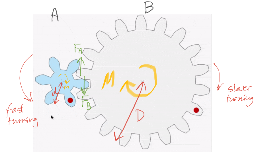
Part 1: A reduction gear arrangement
The driving gear (coloured blue) is smaller and has 6 teeth compared with the large gear’s 18 teeth. This is called a reduction gear arrangement.
A reduction gear arrangement does two things:
It slows down the speed of rotation. You may notice that the large gear turns only one for each three turns of the small gear.
The larger gear exerts a larger moment than the smaller gear. This is because the distance from the centre to the edge is larger for the grey gear.
The blue gear A exerts a force FA on gear B. By Newton’s Third Law, gear B exerts an equal but opposite force FB on gear A. Let’s take the magnitude of both forces to be F.
The anticlockwise moment exerted by gear A is given by m = F x d. The clockwise moment exerted by gear B is given by M=F x D. Since D > d then M > m.
A reduction gear arrangement is typically used in devices like an electric screwdriver. The electric motor in the device produces only a small rotational moment m but a large moment M is needed to turn the screws. The reduction gear produces the large moment M required.
Part 2: The overdrive arrangement
What happens when the driver gear is larger and has a greater number of teeth than the driven gear? This is called an overdrive arrangement.
The example we are going to look at is the arrangement of gears on a bicycle.
Here the driver gear (on the left) is linked via a chain to the smaller driven gear on the right. This means that the anticlockwise moment of the first gear is transmitted directly to the second gear as an anticlockwise moment. That is to say, the direction of the moment is not reversed as it is when the two gears are directly linked by interlocking teeth.
In the example shown, the big gear A turns only once for each four turns completed by the smaller gear B. Let’s assume that gear A exerts a force F on the chain so that the chain exerts an identical force F on gear B. Since D > d, this means that M > m so that the arrangement works as a distance multiplier rather than a force multiplier. This is, of course, excellent if we are riding at speed along a horizontal road. However, if we encounter an upward incline we may wish to — using the gear changing arrangement on the bike — swap the small gear B with one with a larger value of d. This would have the happy effect of increasing the magnitude of m so as to make it slightly easier to pedal uphill.
Rosencrantz (an anguished cry): CONSISTENCY IS ALL I ASK!
Tom Stoppard, Rosencrantz and Guildenstern Are Dead (1966)
I think that dual coding techniques can be extremely helpful in helping students understand the concept of change of momentum.
To engage our students’ physical intuitions, let’s consider a question like: Which would hurt more — being hit by a sandbag or being hit by a rubber ball?
Let’s assume that the sandbag and rubber ball have the same mass m and are travelling at the same initial velocity u. We choose ‘u‘ because it’s the initial velocity and we take ‘v‘ as the final velocity: a very subtle piece of dual coding that can reap rewards if applied consistently — pace Rosencrantz(!) — over a range of disparate examples.
We will use the change = final – initial convention (‘Consistency is all I ask!’)). The initial momentum is piand the final momentum is pf.
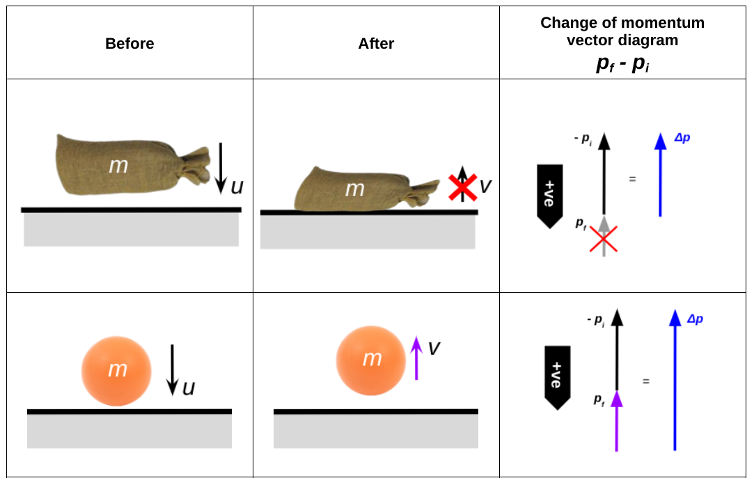
Now let’s work out the change in momentum in each case. We will assume that each item is dropped so that it impacts vertically on a horizontal surface. The velocity just before it hits is u so its initial momentum pi is given by pi = mu; its final velocity is v so its final momentum pf is given by pf = mv. The sandbag does not rebound, so its final velocity v is zero.
The rubber ball rebounds from the surface with a velocity v (we have shown that v < u so we are not assuming a perfectly elastic collision).
We will use the down-is-positive convention so that u is positive and the downward momentum pi are positive in both cases. However, the velocity v of the ball is negative so the momentum pf = mv is negative (upwards).
To add vectors, we simply put them ‘nose to tail’. However, in this case, we need to subtract the vectors, not add them. To do this, we use the operation pf + (-pi,). In other words, we put the vector pf nose to tail with minuspi, or with a vector pointing in the opposite direction to the original vector pi. These are shown in the table.
We can see that the change in momentum Δp is larger in the case of the rubber ball.
Applying Newton Second Law that force = change in momentum / change in time then (assuming the time of each interaction is the same) then we can conclude that the (upward) force exerted by the surface on the ball is larger than the force exerted by the surface on the sandbag.
From Newton’s Third Law (that if an object A exerts a force on object B, then object B exerts an equal and opposite force on object A), we can also conclude that the rubber exerts a larger downward force on the surface. This implies that, if the ball hit (say) your hand, then it would hurt more than the sandbag.
Considering change of momentum problems like this helps students answer questions such as the one shown below:
Exam question on change in momentum (solid black arrow and red arrow added)
We can discard options C and D since the change of momentum shown is in the wrong direction: the vertical component of momentum will remain unchanged.
A and B show changes of momentum of the same magnitude in the horizontal direction. However, if we take the horizontal component of the initial momentum as positive then the change of momentum on the gas particle must be negative; this implies that the correct answer is B.
Note also that diagram B shows the pf + (-pi) operation outlined above, with the arrow showing minus pi shown in red (added to the original exam question).