The worst circuit in the world (part 2)

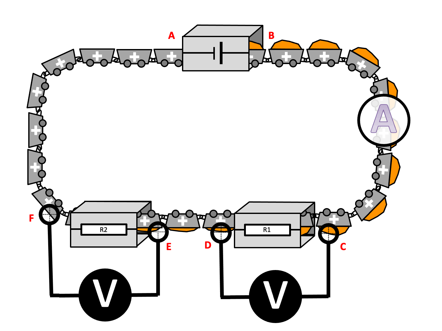
What is the worst circuit in the world? Many teachers think it is the one below.

This is the circuit that AQA (2018: 47) strongly suggest should be used to capture the data for plotting IV characteristics (aka current against potential difference graphs) for a fixed resistor, a filament lamp and a diode. The reasons why it is ‘the worst circuit in world’ were outlined in part one; and also some reasons why, nonetheless, schools teaching the 2016 AQA GCSE Physics / Combined Science specifications should (arguably) continue to use it.

The procedure outlined isn’t ‘perfect’ but works well using the equipment we have available and enables students to capture (and plot using a FREE Excel spreadsheet!) the data with only minor troubleshooting from the teacher.

Step the first: ‘These are the graphs you’re looking for.’

I find this required practical runs more smoothly if students have some awareness of what kind of graphs they are looking for. So, to borrow a phrase, I usually just tell ’em.

You can access an unannotated version of the slides on Google Jamboard and pdf below.

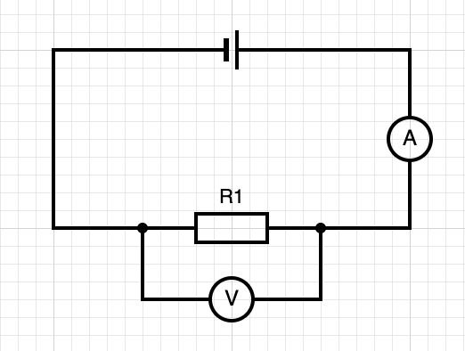
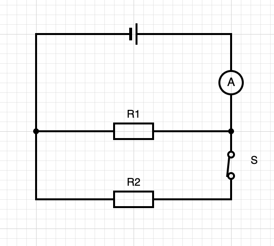
Step the second: capture the data for the fixed resistor

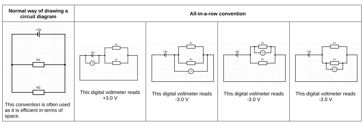
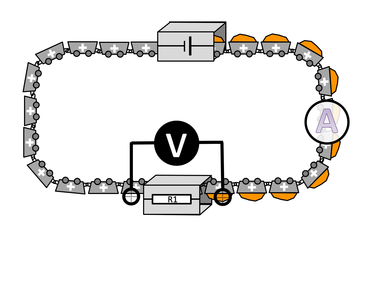
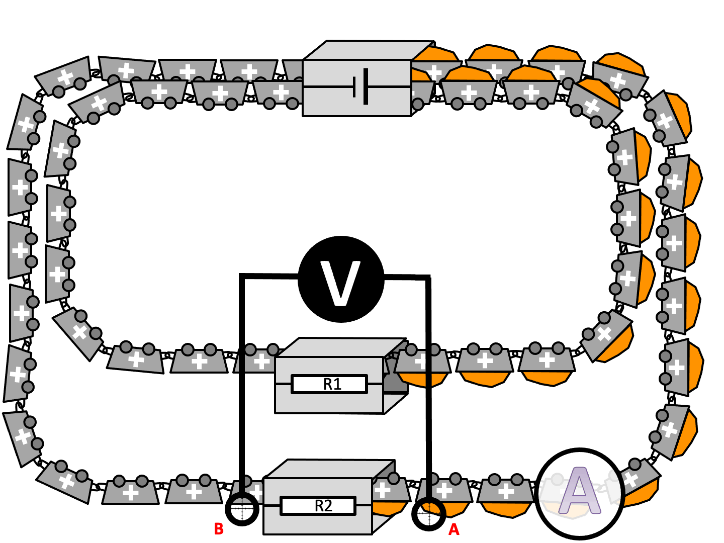
It is a continual source of amazement to me that students seem to find a photograph of a circuit easier to interpret than a nice, clean, minimalist circuit diagram, so for an easier life I present both.

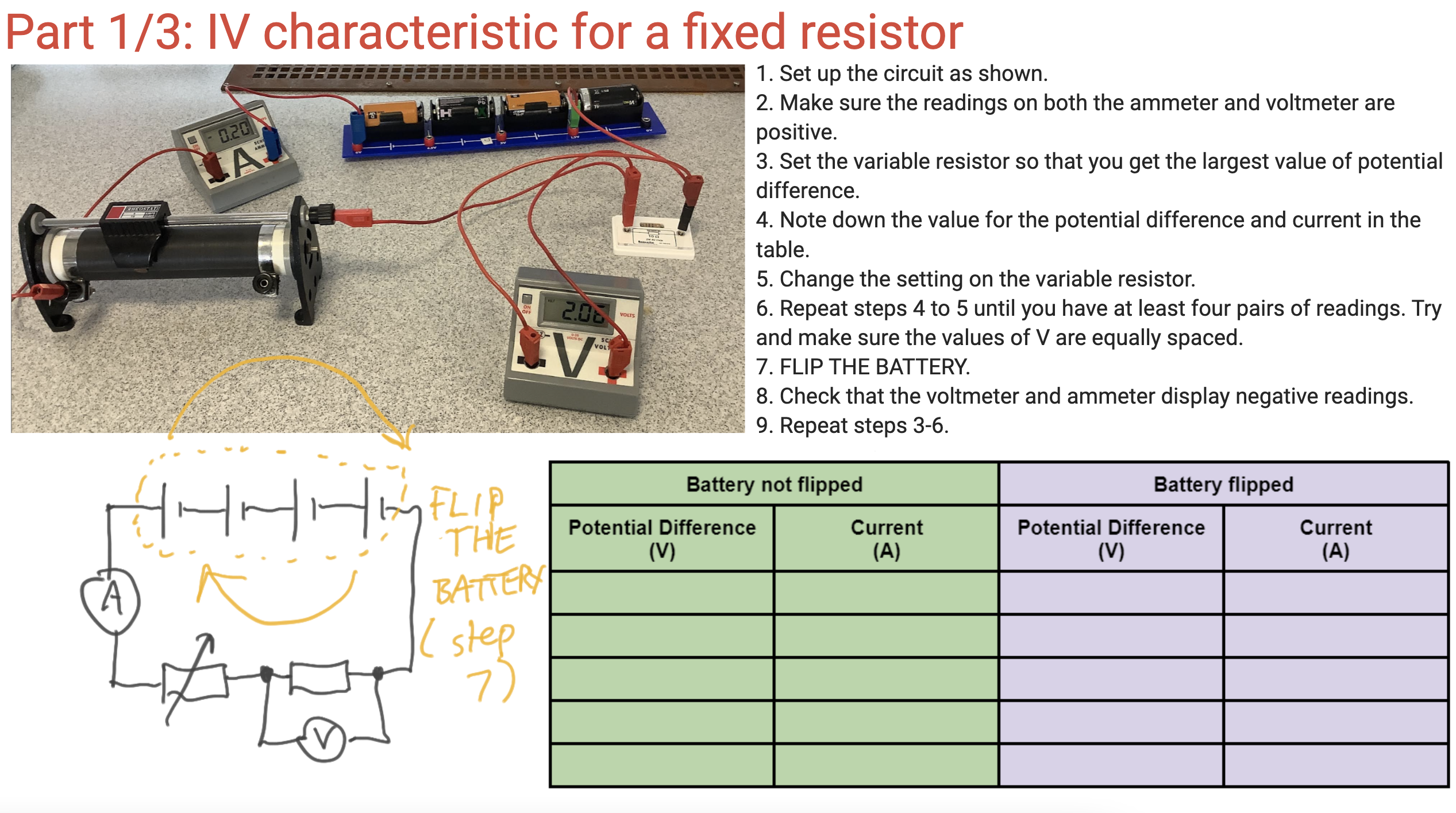
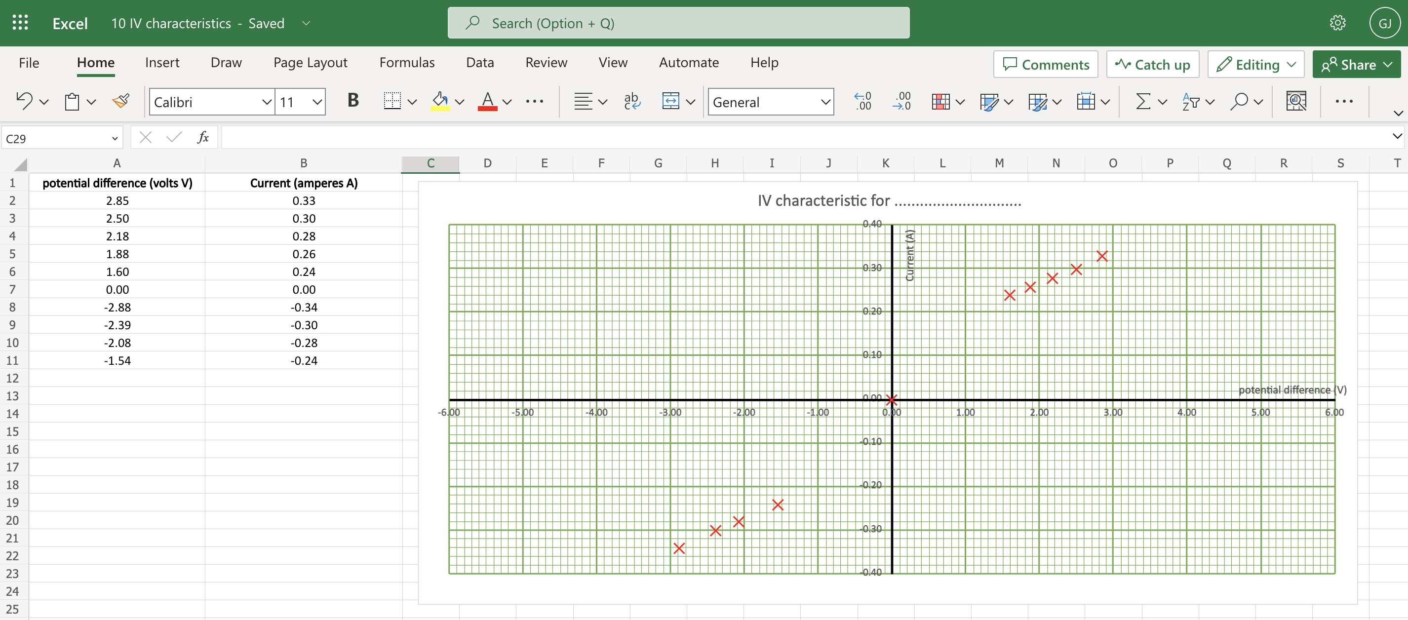
You can, if you have access to ICT, get the students to plot their results ‘live’ on an Excel spreadsheet (link below). I think this is excellent for helping to manage the cognitive demand on our students (as I have argued before here). Please note that I have not used the automated ‘line of best fit’ tools available on Excel as I think it is important for students to practice drawing lines of best fit — including, especially, curved lines of best fit (sorry, Maths teachers, in science there are such things as curved lines!)

Results for a fixed resistor from a typical group of students. These results are clearly consistent with a straight line of best fit going through the origin. However, they can be criticised for not being evenly spaced across the range — but this is a limitation of using the ‘worst circuit in the world’ and, happily(!), gives the students something to write about in their evaluation.

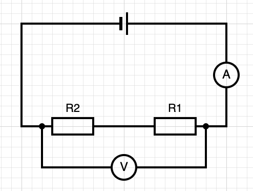
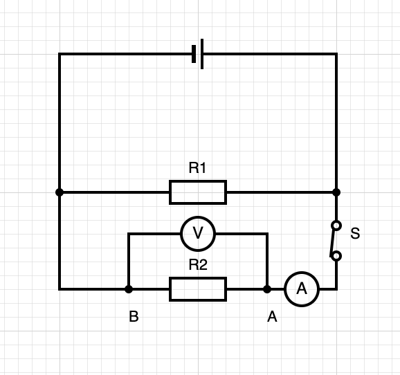
Step the second: capture the data for the filament lamp

In this circuit, we replaced the previous 0-16 ohm variable resistor with a 0 – 1000 ohm variable resistor paired with 2.5 V, 0.2 A filament lamp because the bulb has a resistance of about 60 ohms when run at 2.5 V and so the 0-16 ohm variable resistor is often ineffective. We allowed a maximum potential difference of just over 3.0 V to ‘over run’ the bulb so as to be sure of obtaining the ‘flattening’ of the graph. The method calls for very small adjustments of the variable resistor to obtain noticeable changes of brightness of the bulb. Note that the cells used in the photograph had seen many years of service with our physics department(!) and so were fairly depleted such that three of them were needed to produce a measly three volts; you would likely only need two ‘fresher’, ‘newer’ cells to achieve the same.

These are the results obtained by a typical student group. The results are clearly consistent with the elongated ‘S’ shaped curve predicted from theory. The results can be criticised for clustering, but this can be addressed by students in their evaluation of the experiment.

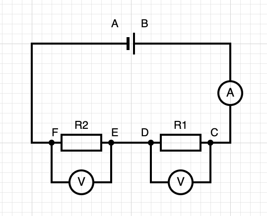
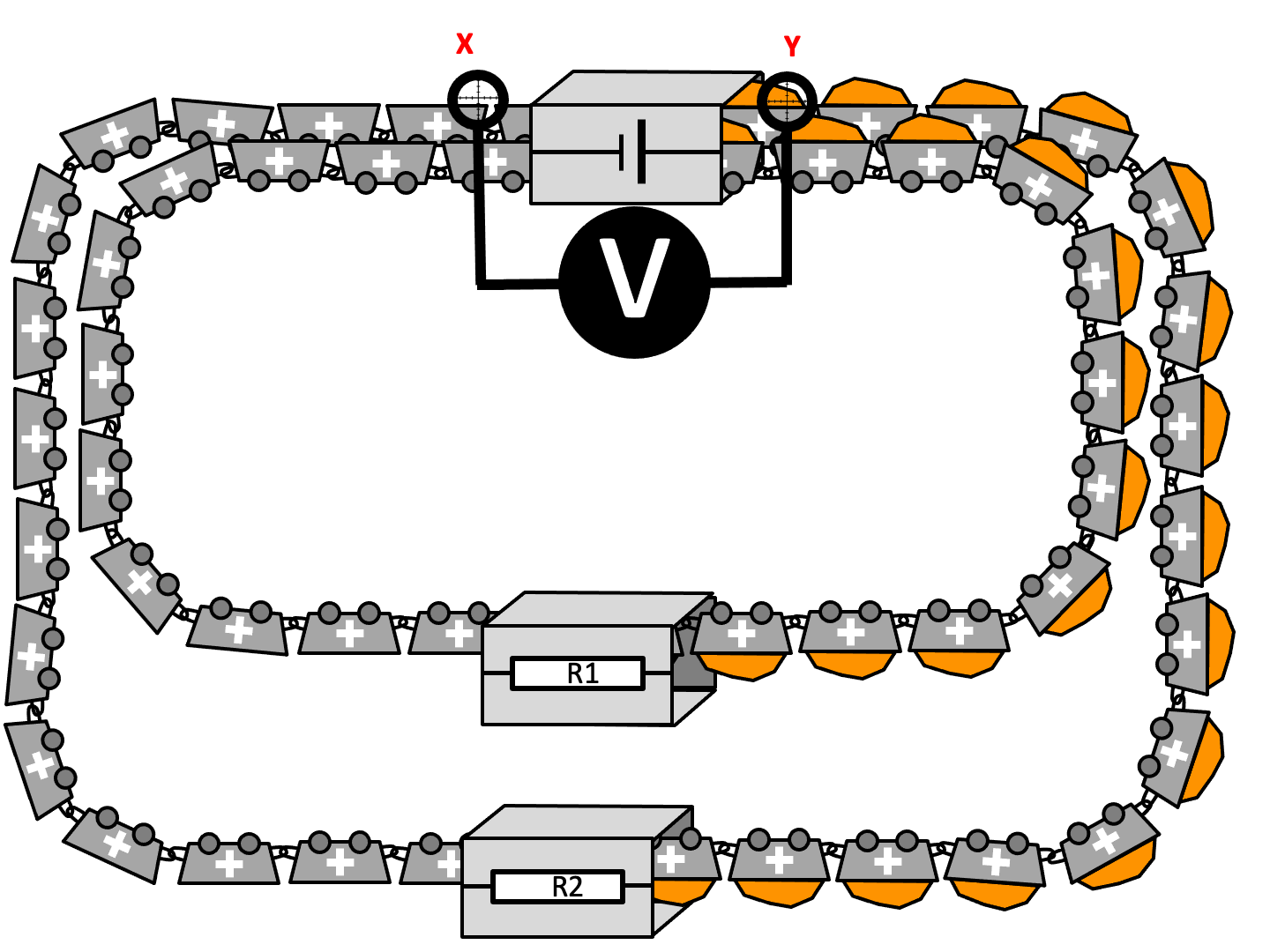
Step the third (sub-parts a and b): capturing the data for a diode

Results for diode captured by a group of students following the procedure outlined above.

Resources

Click here to get a clean copy of the Google Jamboard.

You can download a clean pdf of the slides here:

You can download the Excel spreadsheet used to plot the graphs here:

And, by popular request, a copy of the PowerPoint below (although, trust me, I think Google Jamboard is superior when using ‘live’ in front of a class)

REFERENCES

AQA (2018). Practical Handbook: GCSE Physics. Retrieved from https://filestore.aqa.org.uk/resources/physics/AQA-8463-PRACTICALS-HB.PDF on 7/5/23

The ‘all-in-a-row’ circuit diagram convention for series and parallel circuits

Circuit diagrams can be seen either as pictures or abstractions but it is clear that pupils often find it hard to recognise the circuits in the practical situation of real equipment. Moreover, Caillot found that students retain from their work with diagrams strong images rather than the principles they are intended to establish. The topological arrangement of a diagram or a drawing presents problems for pupils which are easily overlooked. It seems that pupils’ spatial abilities affect their use of circuit diagrams: they sometimes do not regard as identical several circuits, which, though identical, have been rotated so as to have a different spatial arrangement. […] Niedderer found that pupils, when asked whether a circuit diagram would ‘work’ in practice, more often judged symmetrical diagrams to be functioning than non-symmetric ones.

Driver et al. (1994): 124 [Emphases added]

For the reasons outlined by Driver and others above, I think it’s a good idea to vary the way that we present circuit diagrams to students when teaching electric circuits. If students always see circuit diagrams presented so that (say) the cell is at the ‘top’ and ‘facing’ a certain way; or that they are drawn so that they are symmetrical (which is an aesthetic rather that a scientific choice), then they may well incorrectly infer that these and other ‘accidental’ features of our circuit diagrams are the essential aspects that they should pay the most attention to.

One ‘shake it up’ strategy is to redraw a circuit diagram using the ‘all-in-a-row’ convention.

If you arrange the real components in the ‘all-in-a-row’ arrangement, then a standard digital voltmeter has, what is in my opinion a regrettably underused functionality, that will show:

  • ‘positive’ potential differences: that is to say, the energy added to the coulombs as they pass through a cell or the electromotive force; and
  • ‘negative’ potential differences: that is to say, the energy removed from each coulomb as they pass through a resistor; these can be usefully referred to as ‘potential drops’

This can be shown on circuit diagrams as shown below/

In other words, the difference between the potential difference across the cell (energy being transferred into the circuit from the chemical energy store of the cell) is explicitly distinguished from the potential difference across the resistor (energy being transferred from the resistor into the thermal energy store of the surroundings). The all-in-a-row convention neatly sidesteps a common misconception that the potential difference across a cell is equal to the potential difference across a resistor: they are not. While they may be numerically equal, they are different in sign, as a consequence of Kirchoff’s Second Law. As I have suggested before, I think that this misconception is due to the ‘hidden rotation‘ built into standard circuit diagrams.

Potential divider circuits and the all-in-a-row convention

Although I am normally a strong proponent of the ‘parallel first heresy‘, I’ll go with the flow of ‘series circuit first’ in this post.

Diagrams 2 and 3 in the sequence show that the energy supplied to the coulombs (+1.5 V or 1.5 joules per coulomb) by the cell is transferred from the coulombs as they pass through the double resistor combination. Assuming that R1 = R2 then, as diagram 4 shows, 0.75 joules will be transferred out of each coulomb as they pass through R1; as diagram 5 shows, 0.75 joules will be transferred out of each coulomb as they pass through R2.

Parallel circuits and the all-in-a-row convention

I’ve written about using the all-in-a-row convention to help explain current flow in parallel circuits here, so I will focus on understanding potential difference in parallel circuit in this post.

Again, diagrams 2 and 3 in the sequence show that the positive 3.0 V potential difference supplied by the cell is numerically equal (but opposite in sign) to the negative 3.0 V potential drop across the double resistor combination. It is worth bearing in mind that each coulomb passing through the cell gains 3.0 joules of energy from the chemical energy store of the cell. Diagrams 4 and 5 show that each coulomb passing through either R1 or R1 loses its entire 3.0 joules of energy as it passes through that resistor. The all-in-a-row convention is useful, I think, for showing that each coulomb passes through just one resistor as it makes a single journey around the circuit.

Acknowledgements

Circuit simulations from the excellent https://phet.colorado.edu/sims/html/circuit-construction-kit-dc/latest/circuit-construction-kit-dc_en.html

Circuit diagrams drawn using https://www.circuit-diagram.org/editor/

Reference

Driver, R., Squires, A., Rushworth, P., & Wood-Robinson, V. (1994). Making sense of secondary science: Research into children’s ideas. Routledge.

Explaining current flow in conductors (part two)

Do we delve deeply enough into the actual physical mechanism of current flow through electrical conductors using the concepts of charge carriers and electric fields in our treatments for GCSE and A-level Physics? I must reluctantly admit that I am increasingly of the opinion that the answer is no.

In part one we discussed two common misconceptions about the physical mechanism of current flow, namely:

  1. The all-the-electrons-in-a-conductor-repel-each-other misconception; and
  2. The electric-field-of-the-battery-makes-all-the-charge-carriers-in-the-circuit-move misconception.

What, then, does produce the internal electric field that drives charge carriers through a conductor?

Let’s begin by looking at the properties that such a field should have.

Current and electric field in an ohmic conductor

(You can see a more rigorous derivation of this result in Duffin 1980: 161.)

We can see that if we consider an ohmic conductor then for a current flow of uniform current density J we need a uniform electric field E acting in the same direction as J.

What produces the electric field inside a current-carrying conductor?

The electric field that drives charge carriers through a conductor is produced by a gradient of surface charge on the outside of the conductor.

Rings of equal charge density (and the same sign) contribute zero electric field at a location midway between the two rings, whereas rings of unequal charge density (or different sign) contribute a non-zero field at that location.

Sherwood and Chabay (1999): 9

These rings of surface charge produce not only an internal field Enet as shown, but also external fields than can, under the right circumstances, be detected.

Relationship between surface charge densities and the internal electric field

Picture a large capacity parallel plate capacitor discharging through a length of high resistance wire of uniform cross section so that the capacitor takes a long time to discharge. We will consider a significant period of time (a small fraction of RC) when the circuit is in a quasi-steady state with a current density of constant magnitude J. Since E = J / σ then the internal electric field Enet produced by the rings of surface charge must be as shown below.

Schematic diagram showing the relationship between the surface charge density and the internal electric field

In essence, the electric field of the battery polarises the conducting material of the circuit producing a non-uniform arrangement of surface charges. The pattern of surface charges produces an electric field of constant magnitude Enet which drives a current density of constant magnitude J through the circuit.

As Duffin (1980: 167) puts it:

Granted that the currents flowing in wires containing no electromotances [EMFs] are produced by electric fields due to charges, how is it that such a field can follow the tortuous meanderings of typical networks? […] Figure 6.19 shows diagrammatically (1) how a charge density which decreases slowly along the surface of a wire produces an internal E-field along the wire and (2) how a slight excess charge on one side can bend the field into the new direction. Rosser (1970) has shown that no more than an odd electron is needed to bend E around a ninety degree corner in a typical wire.

Rosser suggests that for a current of one amp flowing in a copper wire of cross sectional area of one square millimetre the required charge distribution for a 90 degree turn is 6 x 10⁻³ positive ions per cm3 which they call a “minute charge distribution”.

Observing the internal and external electric fields of a current carrying conductor

Jefimenko (1962) commented that at the time

no generally known methods for demonstrating the structure of the electric field of the current-carrying conductors appear to exist, and the diagrams of these fields can usually be found only in the highly specialized literature. This […] frequently causes the student to remain virtually ignorant of the structure and properties of the electric field inside and, especially, outside the current-carrying conductors of even the simplest geometry.

Jefimenko developed a technique involving transparent conductive ink on glass plates and grass seeds (similar to the classic linear Nuffield A-level Physics electrostatic practical!) to show the internal and external electric field lines associated with current-carrying conductors. Dry grass seeds “line up” with electric field lines in a manner analogous to iron filings and magnetic field lines.

Photograph from Jefimenko (1962: 20). Annotations added

Next post

In part 3, we will analyse the transient processes by which these surface charge distributions are set up.

References

Duffin, W. J. (1980). Electricity and magnetism (3rd ed.). McGraw Hill Book Co.

Jefimenko, O. (1962). Demonstration of the electric fields of current-carrying conductorsAmerican Journal of Physics30(1), 19-21.

Rosser, W. G. V. (1970). Magnitudes of surface charge distributions associated with electric current flow. American Journal of Physics38(2), 265-266.

Sherwood, B. A., & Chabay, R. W. (1999). A unified treatment of electrostatics and circuits. URL http://cil. andrew. cmu. edu/emi. (Note: this article is dated as 2009 on Google Scholar but the text is internally dated as 1999)

Explaining current flow in conductors (part one)

Do we delve deeply enough into the actual physical mechanism of current flow through electrical conductors (in terms of charge carriers and electric fields) in our treatments for GCSE and A-level Physics? I must reluctantly admit that I am increasingly of the opinion that the answer is no.

Of course, as physics teachers we talk with seeming confidence of current, potential difference and resistance but — when push comes to shove — can we (say) explain why a bulb lights up almost instantaneously when a switch several kilometres away is closed when the charge carriers can be shown to be move at a speed comparable to that of a sedate jogger? This would imply a time delay of some tens of minutes between closing the switch and energy being transferred from the power source (via the charge carriers) to the bulb.

When students asked me about this, I tended to suggest one of the following:

  • “The electrons in the wire are repelling each other so when one close to the power source moves, then they all move”; or
  • “Energy is being transferred to each charge carrier via the electric field from the power source.”

However, to be brutally honest, I think such explanations are too tentative and “hand wavy” to be satisfactory. And I also dislike being that well-meaning but unintentionally oh-so-condescending physics teacher who puts a stop to interesting discussions with a twinkly-eyed “Oh you’ll understand that when you study physics at degree level.” (Confession: yes, I have been that teacher too often for comfort. Mea culpa.)

Sherwood and Chabay (1999) argue that an approach to circuit analysis in terms of a predominately classical model of electrostatic charges interacting with electric fields is very helpful:

Students’ tendency to reason locally and sequentially about electric circuits is directly addressed in this new approach. One analyzes dynamically the behaviour of the *whole* circuit, and there is a concrete physical mechanism for how different parts of the circuit interact globally with each other, including the way in which a downstream resistor can affect conditions upstream.

(Side note: I think the Coulomb Train Model — although highly simplified and applicable only to a limited set of “steady state” situations — is consistent with Sherwood and Chabay’s approach, but more on that later.)

Misconception 1: “The electrons in a conductor push each other forwards.”

On this model, the flowing electrons push each other forwards like water molecules pushing neighbouring water molecules through a hose. Each negatively charged electron repels every other negatively charged electron so if one free electron within the conductor moves, then the neighbouring free electrons will also move. Hence, by a chain reaction of mutual repulsion, all the electrons within the conductor will move in lockstep more or less simultaneously.

The problem with this model is that it ignores the presence of the positively charged ions within the metallic conductor. A conveniently arranged chorus-line of isolated electrons would, perhaps, behave analogously to the neighbouring water molecules in a hose pipe. However, as Sherwood and Chabay argue:

Averaged over a few atomic diameters, the interior of the metal is everywhere neutral, and on average the repulsion between flowing electrons is canceled by attraction to positive atomic cores. This is one of the reasons why an analogy between electric current and the flow of water can be misleading.

The flowing electrons inside a wire cannot push each other through the wire, because on average the repulsion by any electron is canceled by the attraction of a nearby positive atomic core (Diagram from Sherwood and Chabay 1999: 4)

Misconception 2: “The charge carriers move because of the electric field from the battery.”

Let’s model the battery as a high-capacity parallel plate capacitor. This will avoid the complexities of having to consider chemical interactions within the cells. Think of a “quasi-steady state” where the current drawn from the capacitor is small so that electric charge on the plates remains approximately constant; alternatively, think of a mechanical charge transfer mechanism similar to the conveyor belt in a Van de Graaff generator which would be able to keep the charge on each plate constant and hence the potential difference across the plates constant (see Sherwood and Chabay 1999: 5).

A representation of the electric field around a single cell battery (modelled as a parallel plate capacitor)

This is not consistent with what we observe. For example, if the charge-carriers-move-due-to-electric-field-of the-battery model was correct then we would expect a bulb closer to the battery to be brighter than a more distant bulb; this would happen because the bulb closer to the battery would be subject to a stronger electric field and so we would expect a larger current.

A bulb closer to the battery is NOT brighter than a bulb further away from the battery (assuming negligible resistance in the connecting wires)

There is the additional argument if we orient the bulb so that the current flow is perpendicular to the electric field line, then there should be no current flow. Instead, we find that the orientation of the bulb relative to the electric field of the battery has zero effect on the brightness of the bulb.

There is no change of brightness as the orientation of the bulb is changed with respect to the electric field lines from the battery

Since we do not observe these effects, we can conclude that the electric field lines from the battery are not solely responsible for the current flow in the circuit.

Understanding the cause of current flow

If the electric field of the battery is not responsible on its own for the potential difference that causes a current to flow, where does the electric field come from?

Interviews reveal that students find the concept of voltage difficult or incomprehensible. It is not known how many students lose interest in physics because they fail to understand basic concepts. This number may be quite high. It is therefore astonishing that this unsatisfactory situation is accepted by most physics teachers and authors of textbooks since an alternative explanation has been known for well over one hundred years. The solution […] was in principle discovered over 150 years ago. In 1852 Wilhelm Weber pointed out that although a current-carrying conductor is overall neutral, it carries different densities of charges on its surface. Recognizing that a potential difference between two points along an electric circuit is related to a difference in surface charges [is the answer].

Härtel (2021): 21

We’ll look at these interesting ideas in part two.

[Note: this post edited 10/7/22 because of a rewritten part two]

References

Härtel, H. (2021). Voltage and Surface ChargesEuropean Journal of Physics Education12(3), 19-31.

Sherwood, B. A., & Chabay, R. W. (1999). A unified treatment of electrostatics and circuits. URL http://cil. andrew. cmu. edu/emi. (Note: this article is dated as 2009 on Google Scholar but the text is internally dated as 1999)

Acknowledgements

The circuit representations were produced using the excellent PhET Sims circuit simulator.

I was “awoken from my dogmatic slumbers” on this topic (and alerted to Sherwood and Chabay’s treatment) by Youtuber Veritasium‘s provocative videos (see here and here).

Series and Parallel Circuits — an unhelpful dichotomy?

Anakin Skywalker and Obi Wan Kenobi discuss the possible unhelpfulness of the concept of ‘series circuits’ and ‘parallel circuits

Are physics teachers following the Way of the Sith? Are we all crossing over to the Dark Side when we talk about ‘series circuits’ and ‘parallel circuits’?

I think that, without meaning to, we may be presenting students with what amounts to a false dichotomy: that all circuits are either series circuits or parallel circuits.

Venn diagram showing the false dichotomy view of series and parallel circuits

The actual situation is more like this:

A Venn diagram showing a more nuanced and realistic view of series and parallel circuits

The confusion may stem from our usage of the word ‘circuit’: are we referring holistically to the entire assemblage of components (highlighted in red) or the individual ‘complete circuits’ (highlighted in green and blue)?

Will the actual ‘circuit’ please stand up? The red circuit is a hybrid circuit, the green circuit is a series circuit, and the blue circuit shows a single resistor in series or parallel with cell (depending on how you look at it)

How to avoid the false dichotomy

I think we should always refer to components in series or components in parallel rather than ‘series circuits’ or ‘parallel circuits’.

Teaching components in parallel using the ‘all-in-a-row’ circuit convention

I’ve written before about what I think is the confusing ‘hidden rotation’ present in normal circuit diagrams. I find redrawing circuit diagrams using the ‘all-in-a-row’ convention useful for explaining circuit behaviour. For simplicity, we’ll assume that all the resistors in the diagrams that follow have a resistance of one ohm.

This can be shown using the Coulomb Train Model like this (coulombs pictured as moving clockwise):

The reason the voltmeter across the cell reads +1.5 V is that energy is being transferred from the chemical energy store of the cell *into* the coulombs. The reason the voltmeter reads -1.5 V across the resistor is that energy is being transferred *from* the coulombs and into the thermal energy store of the resistor.

The current passing through the resistor using I = V/R = 1.5 V / 1 = 1.5 amperes.

Now let’s apply this convention when two resistors are in parallel.

This can be represented using the Coulomb Train Model like this:

I think it’s far clearer that ammeter W is measuring the total current in the circuit while X and Y are measuring the ‘part-current’ passing through R1 and R2 using this convention. (Note: we are assuming that each resistor has a resistance of one ohm.)

Each resistor has a potential difference of -1.5 V because 1.5 J of energy is being shifted from each coulomb as they pass through each resistor.

Also, it is clearer that the cell’s chemical energy store is being drained more quickly when there are two resistors in parallel: two coulombs have to be filled with 1.5 J of energy for each one coulomb in the single resistor circuit.

Thinking about current, the total current in the circuit is 3.0 amperes; so the resistance R = V / I = 1.5 / 3.0 = 0.5 ohms. So two resistors in parallel have a smaller resistance than a single resistor — this is a result that is well worth emphasising for students as so many of them find this completely counterintuitive!

Teaching components in series using the all-in-a-row convention

This circuit can be represented using the Coulomb Train Model like this:

The pattern of potential difference can be explained by looking at the orange ‘energy levels’ carried by each coulomb.

A current of one amp is one coulomb passing per second, so we can see that an ammeter reading would have the same value wherever the ammeter is placed in the circuit.

But look closely at R1: it only has 0.75 V of potential difference across. From I = V/R = 0.75 / 1 = 0.75 amperes.

This means that the total resistance of the circuit from R = V/I is, of course, 2 ohms.

Conclusion

I regret to say that I have probably been teaching ‘series circuits’ and ‘parallel circuits’ on autopilot for much of my career; the same may even be true of some readers of this blog(!)

The Coulomb Train Model has been considered in depth in previous blogs, but I think it’s a good model to encourage students to use their physical intuition (aka ’embodied cognition’) to understand electric circuits.

Whether you agree with the suggested outlines above or not, I hope that it has given you some fruitful food for thought.

The Coulomb Train Model Revisited (Part 5)

In this post, we are going to look at series circuits using the Coulomb Train Model.

The Coulomb Train Model (CTM) is a helpful model for both explaining and predicting the behaviour of real electric circuits which I think is useful for KS3 and KS4 students.

Without further ado, here is a a summary.


A circuit with one resistor

Let’s look at a very simple circuit to begin with:

This can be represented on the CTM like this:

The ammeter counts 5 coulombs passing every 10 seconds, so the current I = charge flow Q / time t = 5 coulombs / 10 seconds = 0.5 amperes.

We assume that the cell has a potential difference of 1.5 V so there is a potential difference of 1.5 V across the resistor R1 (that is to say, each coulomb loses 1.5 J of energy as it passes through R1).

The resistor R1 = potential difference V / current I = 1.5 / 0.5 = 3.0 ohms.


A circuit with two resistors in series

Now let’s add a second identical resistor R2 into the circuit.

This can be shown using the CTM like this:

Notice that the current in this example is smaller than in the first circuit; that is to say, fewer coulombs go through the ammeter in the same time. This is because we have added a second resistor and remember that resistance is a property that reduces the current. (Try and avoid talking about a high resistance ‘slowing down’ the current because in many instances such as two conductors in parallel a high current can be modelled with no change in the speed of the coulombs.)

Notice also that the voltmeter is making identical measurements on both the circuit diagram and the CTM animation. It is measuring the total energy change of the coulombs as they pass through both R1 and R2.

The current I = charge flow Q / time t = 5 coulombs / 20 seconds = 0.25 amps. This is half the value of the current in the first circuit.

We have an identical cell of potential difference 1.5 V the voltmeter would measure 1.5 V. We can calculate the total resistance using R = V / I = 1.5 / 0.25 = 6.0 ohms.

This is to be expected since the total resistance R = R1 + R2 and R1 = 3.0 ohms and R2 = 3.0 ohms.


Looking at the resistors individually

The above circuit can be represented using the CTM as follows:

Between A and B, the coulombs are each gaining 1.5 joules since the cell has a potential difference of 1.5 V. (Remember that V = E energy transferred (in joules) / Q charge flow (in coulombs.)

Between B and C the coulombs lose no energy; that is to say, we are assuming that the connecting wires have negligible resistance.

Between C and D the coulombs lose some energy. We can use the familar V = I x R to calculate how much energy is lost from each coulomb, since we know that R1 is 3.0 ohms and I is 0.25 amperes (see previous section).

V = I x R = 0.25 x 3.0 = 0.75 volts.

That is to say, 0.75 joules are removed from each coulomb as they pass through R1 which means that (since 1.5 joules were added to each coulomb by the cell) that 0.75 joules are left in each coulomb.

The coulombs do not lose any energy travelling between D and E because, again, we are assuming negligible resistance in the connecting wire.

0.75 joules is removed from each coulomb between E and F making the potential difference across R2 to be 0.75 volts.

Thus we find that the familiar V = V1 + V2 is a direct consequence of the Principle of Conservation of Energy.


FAQ: ‘How do the coulombs know to drop off only half their energy in R1?’

Simple answer: they don’t.

This may be a valid objection for some donation models of electric circuits (such as the pizza delivery van model) but it doesn’t apply to the CTM because it is a continuous chain model (with the caveat that the CTM applies only to ‘steady state’ circuits where the current is constant).

Let’s look at a numerical argument to support this:

  • The magnitude of the current is controlled by only two factors: the potential difference of the cell and the total resistance of the circuit.
  • In other words, if we increased the value of R1 to (say) 4 ohms and reduced the value of R2 to 2 ohms so that the total resistance was still 6 ohms, the current would still be 0.25 amps.
  • However, in this case the energy dissipated by each coulomb passing through R1 would V = I x R = 0.25 x 4 = 1 volt (or 1 joule per coulomb) and similarly the potential difference across R2 would now be 0.5 volts.
  • The coulombs do not ‘know’ to drop off 1 joule at R1 and 0.5 joules at R2: rather, it is a purely mechanical interaction between the moving coulombs and each resistor.
  • R1 has a bigger proportion of the total resistance of the circuit than R2 so it seems self-evident (at least to me) that the coulombs will lose a larger proportion of their total energy passing through R1.
  • A similar analysis would apply if we made R2 = 4 ohms and R1 = 2 ohms: the coulombs would now lose 0.5 joules passing through R1 and 1 joule passing through R2.

Thus, we see that the current in a series circuit is affected by the ‘global’ or ‘whole circuit’ properties such as the potential difference of the cell and the total resistance of the circuit. The CTM models this property of real circuits by being a continuous chain of mechanically-linked ‘trucks’ so that a change in any one part of the circuit affects the movement of all the coulombs.

However, the proportion of the energy lost by a coulomb travelling through one part of the circuit is affected — not by ‘magic’ or a weird form of ‘coulomb telepathy’ — but only by the ‘local’ properties of that section of the circuit i.e. the electrical resistance of that section.

The CTM analogue of a low resistance section of a circuit (top) and a high resistance section of a circuit (bottom)

(PS You can read more about the CTM and potential divider circuits here.)


Afterword

You may be relieved to hear that this is the last post in my series on ‘The CTM revisited’. My thanks to the readers who have stayed with me through the series (!)

I will close by saying that I have appreciated both the expressions of enthusiasm about CTM and the thoughtful criticisms of it.

The Coulomb Train Model Revisited (Part 4)

In this post, we will look at parallel circuits.

The Coulomb Train Model (CTM) is a helpful model for both explaining and predicting the behaviour of real electric circuits which I think is useful for KS3 and KS4 students.

Without further ado, here is a a summary.

This is part 4 of a continuing series. (Click to read Part 1, Part 2 or Part 3.)


The ‘Parallel First’ Heresy

I advocate teaching parallel circuits before teaching series circuits. This, I must confess, sometimes makes me feel like Captain Rum from Blackadder Two:

The main reason for this is that parallel circuits are conceptually easier to analyse than series circuits because you can do so using a relatively naive notion of ‘flow’ and gives students an opportunity to explore and apply the recently-introduced concept of ‘flow of charge’ in a straightforward context.

Redish and Kuo (2015: 584) argue that ‘flow’ is an example of embodied cognition in the sense that its meaning is grounded in physical experience:

The thesis of embodied cognition states that ultimately our conceptual system grounded in our interaction with the physical world: How we construe even highly abstract meaning is constrained by and is often derived from our very concrete experiences in the physical world.

Redish and Kuo (2015: 569)

As an aside, I would mention that Redish and Kuo (2015) is an enduringly fascinating paper with a wealth of insights for any teacher of physics and I would strongly recommend that everyone reads it (see link in the Reference section).


Let’s Go Parallel First — but not yet

Let’s start with a very simple circuit.

This is not a parallel circuit (yet) because switch S is open. Resistors R1 and R2 are identical.

This can be represented on the coulomb train model like this:

Five coulombs pass through the ammeter in 20 seconds so the current I = Q/t = 5/20 = 0.25 amperes.

Let’s assume we have a 1.5 V cell so 1.5 joules of energy are added to each coulomb as they pass through the cell. Let’s also assume that we have negligible resistance in the cell and the connecting wires so 1.5 joules of energy will be removed from each coulomb as they pass through the resistor. The voltmeter as shown will read 1.5 volts.

The resistance of the resistor R1 is R=V/I = 1.5/0.25 = 6.0 ohms.


Let’s Go Parallel First — for real this time.

Now let’s close switch S.

This is example of changing an example by continuous conversion which removes the need for multiple ammeters in the circuit. The changed circuit can be represented on the CTM as shown

Now, ten coulombs pass through the ammeter in twenty seconds so I = Q/t = 10/20 = 0.5 amperes (double the reading in the first circuit shown).

Questioning may be useful at this point to reinforce the ‘flow’ paradigm that we hope students will be using:

  • What will be the reading if the ammeter moved to a similar position on the other side? (0.5 amps since current is not ‘used up’.)
  • What would be the reading if the ammeter was placed just before resistor R1? (0.25 amps since only half the current goes through R1.)

To calculate the total resistance of the whole circuit we use R = V/I = 1.5/0.5 = 3.0 ohms– which is half of the value of the circuit with just R1. Adding resistors in parallel has the surprising result of reducing the total resistance of the circuit.

This is a concrete example which helps students understand the concept of resistance as a property which reduces current: the current is larger when a second resistor is added so the total resistance must be smaller. Students often struggle with the idea of inverse relationships (i.e. as x increases y decreases and vice versa) so this is a point well worth emphasising.


Potential Difference and Parallel Circuits (1)

Let’s expand on the primitive ‘flow’ model we have been using until now and adapt the circuit a little bit.

This can be represented on the CTM like this:

Each coulomb passing through R2 loses 1.5 joules of energy so the voltmeter would read 1.5 volts.

One other point worth making is that the resistance of R2 (and R1) individually is still R = V/I = 1.5/0.25 = 6.0 ohms: it is only the combined effect of R1 and R2 together in parallel that reduces the total resistance of the circuit.


Potential Difference and Parallel Circuits (2)

Let’s have one last look at a different aspect of this circuit.

This can be represented on the CTM like this:

Each coulomb passing through the cell from X to Y gains 1.5 joules of energy, so the voltmeter would read 1.5 volts.

However, since we have twice the number of coulombs passing through the cell as when switch S is open, then the cell has to load twice as many coulombs with 1.5 joules in the same time.

This means that, although the potential difference is still 1.5 volts, the cell is working twice as hard.

The result of this is that the cell’s chemical energy store will be depleted more quickly when switch S is closed: parallel circuits will make cells go ‘flat’ in a much shorter time compared with a similar series circuit.

Bulbs in parallel may shine brighter (at least in terms of total brightness rather than individual brightness) but they won’t burn for as long.

To some ways of thinking, a parallel circuit with two bulbs is very much like burning a candle at both ends…


More fun and high jinks with coulomb train model in the next instalment when we will look at series circuits.

You can read part 5 here.


Reference

Redish, E. F., & Kuo, E. (2015). Language of physics, language of math: Disciplinary culture and dynamic epistemologyScience & Education24(5), 561-590.

The Coulomb Train Model Revisited (Part 3)

In this post, we will look at explaining electrical resistance using the Coulomb Train Model.

This is part 3 of a continuing series (click to read part 1 and part 2).

The Coulomb Train Model (CTM) is a helpful model for both explaining and predicting the behaviour of real electric circuits which I think is useful for KS3 and KS4 students.

Without further ado, here is a a summary.

A summary of the Coulomb Train Model

Representing Resistance on the CTM

To measure resistance, we would set up this circuit.

We can represent this same circuit on the CTM as follows:

If we count how many ‘coulombs’ (grey trucks) pass one point in a certain time then on this animation we get 5 coulombs in 20 seconds.
This is equivalent to a current of
5 coulombs / 20 seconds = 0.2 coulombs per second = 0.2 amperes.

This way of thinking about current is consistent with the formula charge flow = current x time or Q=It which can be rearranged to give I=Q/t.

We have used identical labels on the circuit diagram and the CTM animation to encourage students to view them as different representations of a real situation. The ammeter at X would read 0.2 amps. We could place the ammeter at any other point in the circuit and still get a reading of 0.2 amps since ammeters only ‘count coulombs per second’ and don’t make any measurement of energy (represented by the orange substance in the trucks).

However, the voltmeter does make a measurement of energy: it compares the energy difference between a single coulomb at Y and a single coulomb at Z. If (say) 1.5 joules of energy is transferred from each coulomb as it passes through the bulb from Y to Z then the voltmeter will read a potential difference (or ‘voltage’ if you prefer) of 1.5 volts.

This way of thinking about potential difference is consistent with the formula energy transferred = charge flow x potential difference or E=QV which we can rearrange to give V=E/Q.

So as you can see, one volt is really equivalent to an energy change of one joule for every coulomb (!)

We can calculate the resistance of the bulb by using R=V/I so R = 1.5/0.2 = 7.5 ohms.


Resistance is not futile . . .

Students sometimes have difficulty accepting the idea of a ‘resistor’: ‘Why would anyone in their right minds deliberately design something that reduces the flow of electric current?’ It’s important to explain that it is vital to be able to control the flow of electric current and that one of the most common electronic components in your phone or games console is — the humble resistor.

One of many resistors on a circuit board. The colour codes tell us the value of each resistor.

Teachers often default to explaining electric circuits using bulbs as the active component. There is a lot to recommend this practice, not least the fact that changes in the circuit instantaneously affect the brightness of the bulb. However, it vital (especially at GCSE) to allow students to learn about circuits featuring resistors and other components rather than just the pedagogically overused (imho) filament lamp.


Calculating the resistance of a resistor

Consider this circuit where we have a resistor R1.

This can be represented as a coulomb train model like this:

The resistor does not glow with visible light as the bulb does, but it would glow pretty brightly if viewed through an infra red camera since the energy carried by the coulombs is transferred to the thermal energy store of the resistor. The only way we can observe this energy shift without such a special camera is to use a voltmeter.

Let’s begin by analysing this circuit qualitatively.

  • The coulombs are moving faster in this circuit than the previous circuit. This means that the current is larger. (Remember: current is coulombs per second.)
  • Because the current is larger, R1 must have a smaller resistance than the bulb. (Remember: resistance is a quantity that reduces the current.)
  • The energy transferred to each coulomb is the same in each example so the potential difference of the cell is the same in both circuits. (Of course, V can be altered by adding a second cell or turning up the setting on a power supply, but in many circuits V is, loosely speaking, a ‘fixed’ or ‘quasi-constant’ value.)
  • Because the ‘push’ or potential difference is the same size but the resistance of R1 is smaller, then the same cell is able to push a larger current around the circuit.

Now let’s analyse the circuit quantitatively.

  • 5 coulombs pass a single point in 13 seconds so the current is 5/13 = 0.38 coulombs per second = 0.4 amperes. (Double the current in the bulb circuit.)
  • The resistance can be calculated using R=V/I = 1.5/0.4 = 3.75 ohms. (Half the resistance of the bulb.)
  • Each coulomb is being loaded with 1.5 J of energy as it passes through the cell. Since this is happening twice as often in the resistor circuit as the bulb circuit, the cell will ‘go flat’ or ’empty its chemical energy store’ in half the time of the bulb cell.

So there we have it: more fun and high jinks with the CTM.

I hope that I have persuaded a few more teachers that the CTM is useful for getting students to think productively and, more importantly, quantitatively using correct scientific terminology about electric circuits.

In the next installment, we will look at series and parallel circuits.

The Coulomb Train Model Revisited (Part 1)

The Coulomb Train Model (CTM) is a helpful model for both explaining and predicting the behaviour of real electric circuits which I think is suitable for use with KS3 and KS4 students (that’s 11-16 year olds for non-UK educators).

I have written about it before (see here and here) but I have recently been experimenting with animated versions of the original diagrams.

Essentially, the CTM is a donation model akin to the famous ‘bread and bakery van’ or even the ‘penguins and ski lift’ models, but to my mind it has some major advantages over these:

  • The trucks (‘coulombs’) in the CTM are linked in a continuous chain. If one ‘coulomb’ stops then they all stop. This helps students grasp why a break anywhere in a circuit will stop all current.
  • The CTM presents a simplified but still quantitatively accurate picture of otherwise abstract entities such as coulombs and energy rather than the more whimsical ‘bread van’ = ‘charge carrier’ and ‘bread’ = ‘energy’ (or ‘penguin’ = ‘charge carrier’ and ‘gpe of penguin’ = ‘energy of charge carrier’) for the other models.
  • Explanations and predictions scripted using the CTM use direct but substantially correct terminiology such as ‘One ampere is one coulomb per second’ rather than the woolier ‘current is proportional to the number of bread vans passing in one second’ or similar.

Modelling current flow using the CTM

The coulombs are the ‘trucks’ travelling clockwise in this animation. This models conventional current.

Charge flow (in coulombs) = current (in amps) x time (in seconds)

So a current of one ampere is one coulomb passing in one second. On the animation, 5 coulombs pass through the ammeter in 25 seconds so this is a current of 0.20 amps.

We have shown two ammeters to emphasise that current is conserved. That is to say, the coulombs are not ‘used up’ as they pass through the bulb.

The ammeters are shown as semi-transparent as a reminder that an ammeter is a ‘low resistance’ instrument.


Modelling ‘a source of potential difference is needed to make current flow’ using the CTM

Energy transferred (in joules) = potential difference (in volts) x charge flow (in coulombs) 

So the potential difference = energy transferred divided by the number of coulombs.

The source of potential difference is the number of joules transferred into each coulomb as it passes through the cell. If it was a 1.5 V cell then 1.5 joules of energy would be transferred into each coulomb.

This is represented as the orange stuff in the coulombs on the animation.

What is this energy? Well, it’s not ‘electrical energy’ for certain as that is not included on the IoP Energy Stores and Pathways model. In a metallic conductor, it would be the sum of the kinetic energy stores and electrical potential energy stores of 6.25 billion billion electrons that make up one coulomb of charge. The sum would be a constant value (assuming zero resistance) but it would be interchanged randomly between the kinetic and potential energy stores.

For the CTM, we can be a good deal less specific: it’s just ‘energy’ and the CTM provides a simplified, concrete picture that allows us to apply the potential difference equation in a way that is consistent with reality.

Or at least, that would be my argument.

The voltmeter is shown connected in parallel and the ‘gloves’ hint at it being a ‘high resistance’ instrument.

More will follow in part 2 (including why I decided to have the bulb flash between bright and dim in the animations).

You can read part 2 here.