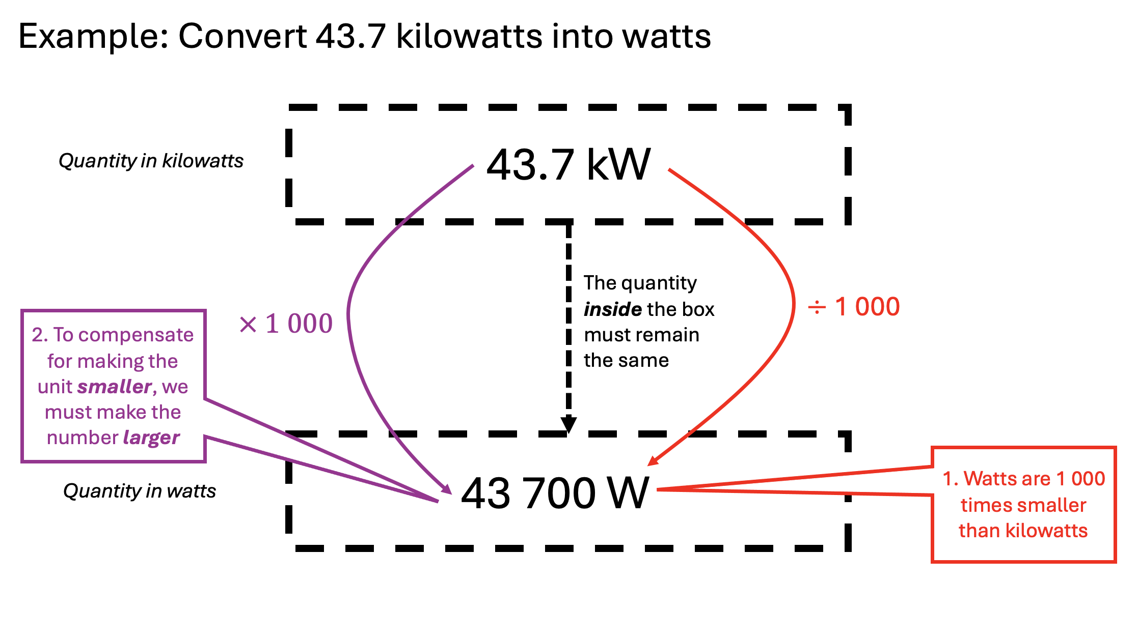
As I have written before, many students struggle with unit conversions. The Porter Method helps students’ understanding by making the process explicit.
Using the Porter Method to explain the mysteries of unit conversions
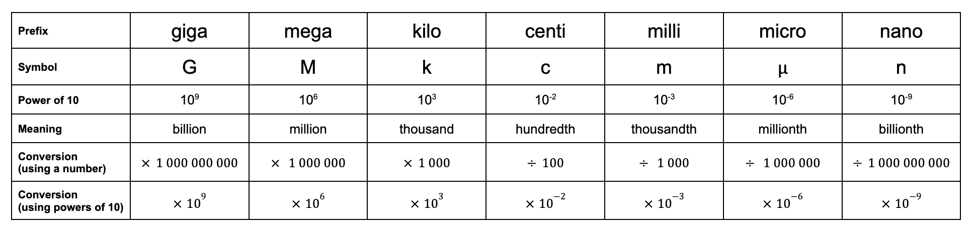
As of the time of writing, GCSE Science (2015 specification) students are expected to know the SI unit prefixes from giga- to nano-.
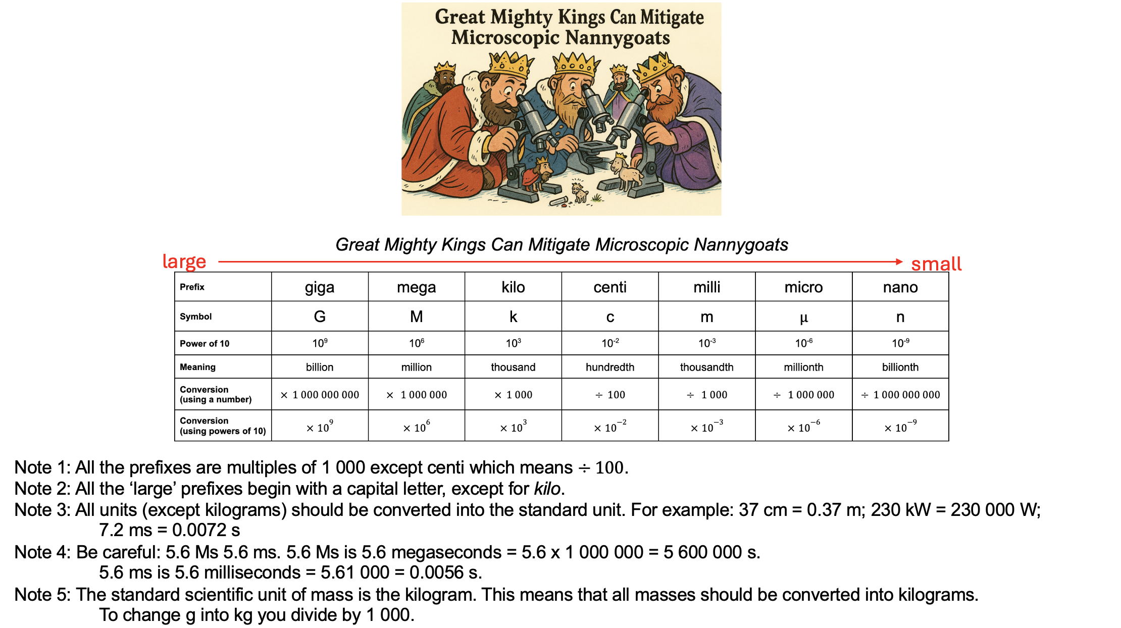
I suggest the following mnemonic:
A mnemonic for memorising the SI unit prefixes needed for GCSE
Choosing a mnemonic can be difficult because ‘mega’, ‘milli’ and ‘micro’ all begin with m, and even the first two letters of ‘milli’ and ‘micro’ are both ‘mi’. The mnemonic about helps students remember the difference between ‘milli’ and ‘micro’ by using ‘microscopic’ to help.
If you think this approach will be useful for your students, the Powerpoint is attached.
Enjoy!
PS You can find more of my thoughts on the SI system here
What is the worst circuit in the world? Many teachers think it is the one below.
This is the circuit that AQA (2018: 47) strongly suggest should be used to capture the data for plotting IV characteristics (aka current against potential difference graphs) for a fixed resistor, a filament lamp and a diode. The reasons why it is ‘the worst circuit in world’ were outlined in part one; and also some reasons why, nonetheless, schools teaching the 2016 AQA GCSE Physics / Combined Science specifications should (arguably) continue to use it.
The procedure outlined isn’t ‘perfect’ but works well using the equipment we have available and enables students to capture (and plot using a FREE Excel spreadsheet!) the data with only minor troubleshooting from the teacher.
Step the first: ‘These are the graphs you’re looking for.’
I find this required practical runs more smoothly if students have some awareness of what kind of graphs they are looking for. So, to borrow a phrase, I usually just tell ’em.
You can access an unannotated version of the slides on Google Jamboard and pdf below.
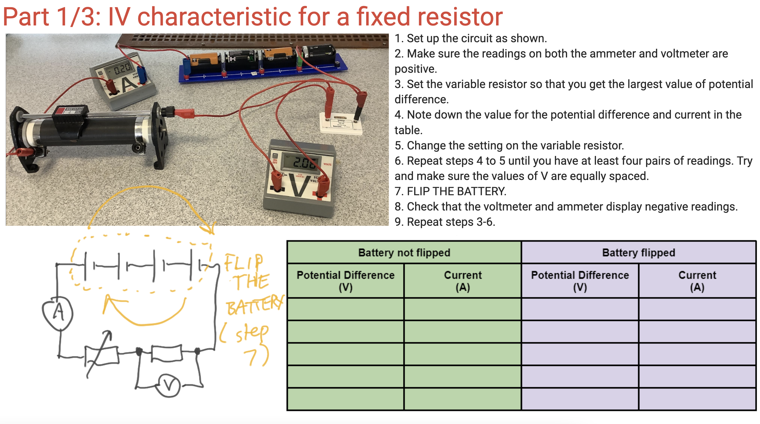
Step the second: capture the data for the fixed resistor
It is a continual source of amazement to me that students seem to find a photograph of a circuit easier to interpret than a nice, clean, minimalist circuit diagram, so for an easier life I present both.
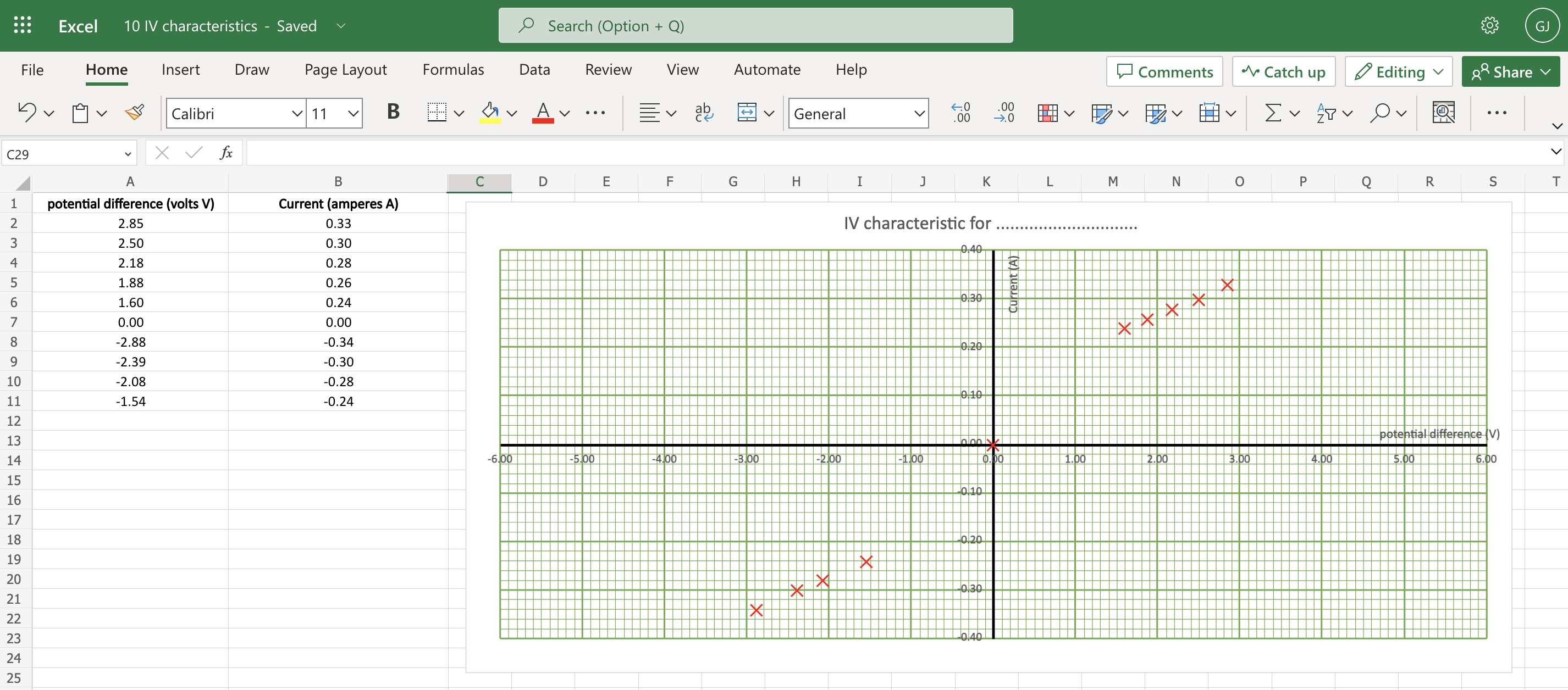
You can, if you have access to ICT, get the students to plot their results ‘live’ on an Excel spreadsheet (link below). I think this is excellent for helping to manage the cognitive demand on our students (as I have argued before here). Please note that I have not used the automated ‘line of best fit’ tools available on Excel as I think it is important for students to practice drawing lines of best fit — including, especially, curved lines of best fit (sorry, Maths teachers, in science there are such things as curved lines!)
Results for a fixed resistor from a typical group of students. These results are clearly consistent with a straight line of best fit going through the origin. However, they can be criticised for not being evenly spaced across the range — but this is a limitation of using the ‘worst circuit in the world’ and, happily(!), gives the students something to write about in their evaluation.
Step the second: capture the data for the filament lamp
In this circuit, we replaced the previous 0-16 ohm variable resistor with a 0 – 1000 ohm variable resistor paired with 2.5 V, 0.2 A filament lamp because the bulb has a resistance of about 60 ohms when run at 2.5 V and so the 0-16 ohm variable resistor is often ineffective. We allowed a maximum potential difference of just over 3.0 V to ‘over run’ the bulb so as to be sure of obtaining the ‘flattening’ of the graph. The method calls for very small adjustments of the variable resistor to obtain noticeable changes of brightness of the bulb. Note that the cells used in the photograph had seen many years of service with our physics department(!) and so were fairly depleted such that three of them were needed to produce a measly three volts; you would likely only need two ‘fresher’, ‘newer’ cells to achieve the same.
These are the results obtained by a typical student group. The results are clearly consistent with the elongated ‘S’ shaped curve predicted from theory. The results can be criticised for clustering, but this can be addressed by students in their evaluation of the experiment.
Step the third (sub-parts a and b): capturing the data for a diode
Results for diode captured by a group of students following the procedure outlined above.
And, by popular request, a copy of the PowerPoint below (although, trust me, I think Google Jamboard is superior when using ‘live’ in front of a class)
It is a truth which is by no means universally acknowledged, but one of which I hope shortly to persuade the reader, that introducing speed to 11-14 year-old students as speed=distance÷time or s=d ÷ t is not the most pedagogically effective approach.
This may initially seem like perverse idea since surely s = d ÷ t and s × t = d are mathematically equivalent expressions? They are, but it is my contention that many students find expressions of the format s = d ÷ t more cognitively demanding that s×t=d. This is because many students struggle with the concept of inverse relationships, particularly those involving multiplication and division.
[Researchers have] suggested that multiplicative concepts may be more difficult to acquire than additive ones, and speculated that although addition and subtraction concepts and procedures extend to multiplication and division, the latter also include unique aspects unrelated to addition and subtraction.
Robinson and LeFevre 2012: 426
In short, many students can handle solving problems such as a + b = c where (say) the numerical values of b and c are known. This can be solved by performing the operation a + b – b = c – b leading to a = c – b and hence a solution to the problem. However, students — and many adults(!) — find solving a similar problem of the format a=b÷c much more problematic, especially in cases when b÷c is not a simple integer.
Compounding students’ inability to utilise multiplicative structures, is their failure to recognise the isomorphism between proportion problems. Another possible reason is that a reluctance or inability to deal with the non-integer relationships (‘avoidance of fractions’), coupled with the high processing loads involved, seems to be the likely cause of this error
Singh 2000: 595
The problem with the s=d÷t format
In this analysis, we will assume that a direct calculation of s when d and t are known is trivial. The problem with the s=d÷t format is that it may require students to apply two problem solving procedures which, to the novice learner, have highly dissimilar surface features and whose underlying isomorphism is, therefore, hidden from them.
To find d if s and t are known, they need to multiply both sides by t (see Example 1).
To find t if s and d are known, they need to divide both sides by s and then multiply both sides by t (see Example 2)
Example 1
Example 2
(For more on using the ‘FIFA’ mnemonic for calculations, click on this link.)
Easing cognitive load with the s x t = d format
As above, we will assume that a direct calculation of d when s and t are known is trivial. What happens when we need to find s and t, given that they are the only unknown quantities?
If t and d are known, then we can find s by dividing both sides by t (see Example 3).
If s and t are known, then we can find t by dividing both sides s (see Example 4).
Example 3
Example 4
Examples 3 and 4 have highly similar surface features as well as a deeper level isomorphism and allow a commonality of approach which I think is immensely helpful for novice learners.
Robinson and LeFevre (2012: 411) call this type of operation ‘the inversion shortcut’ and argue (for a different context than the one presented here) that:
In three-term problems such as a × b ÷ b, the knowledge that b ÷ b = 1, combined with the associative property of multiplication, allows solvers to implement an inversion shortcut on problems such as 4×24÷24. The computational advantage of using the inversion shortcut is dramatic, resulting in greatly reduced solution times and error rates relative to a left-to-right solution procedure. […] Such knowledge of how inverse operations relate in a variety of circumstances forms the basis for understanding and manipulating algebraic expressions, an important mathematical activity for adolescents
Conclusion
I think there is a strong case to be made for this mode of presentation to be applied to a wider range of physics contexts for 11-16 year-old students such as:
Power, so that the definition of power is initially presented as P × t = E or P × t = W; that is to say, we define power as the energy transferred in one second.
Density, so that ρ × V = m; that is to say, we define density as mass of 1 m3 or 1 cm3.
Pressure, so that the definition of pressure is initially presented as p × A = F; that is to say, we define pressure as the force exerted on an area of 1 metre squared.
Acceleration, so that a × t = Δv; that is to say, we define acceleration as the change in velocity produced in one second.
Please feel free to leave a comment
References
Robinson, K. M., & LeFevre, J. A. (2012). The inverse relation between multiplication and division: Concepts, procedures, and a cognitive framework. Educational Studies in Mathematics, 79(3), 409-428.
Singh, P. (2000). Understanding the concepts of proportion and ratio among grade nine students in Malaysia. International Journal of Mathematical Education in Science and Technology, 31(4), 579-599.
I recently made a bit of a mess of teaching the topic of gears by trying to ‘wing it’ with insufficient preparation. To avoid my — and possibly others’ — future blushes, I thought I would compile a post summarising my interpretation of what students need to know about gears for AQA GCSE Physics.
I am going to include some handy gifs and a clean, un-annotated Google Jamboard (my favoured medium for lessons).
Any continuing errors, omissions or misconceptions are entirely my own fault.
‘A simple gear system can be used to transmit the rotational effect of a force’ [AQA 4.5.4]
A gear is a wheel with teeth that can transmit the rotational effect of a force.
For example, in the gear train shown above, the first gear (A) is turned by a motor (green dot shown below). The moment (rotational effect) is passed via the interlocking teeth to gear B and so on down the chain to gear E. It is also worth pointing out that gear A has a clockwise moment but gear B has an anticlockwise moment. The direction alternates as we move down the chain. It takes a gear train of five gears to transmit the clockwise moment from gear A to gear E.
Gears A-E are all equal in size with the same number of teeth and, consequently, the moment does not change in magnitude as it passes down the chain (although, as noted above, it does change direction from clockwise to anticlockwise).
‘Students should be able to explain how gears transmit the rotational effect of forces’ [AQA 4.5.4]
Part 1: A reduction gear arrangement
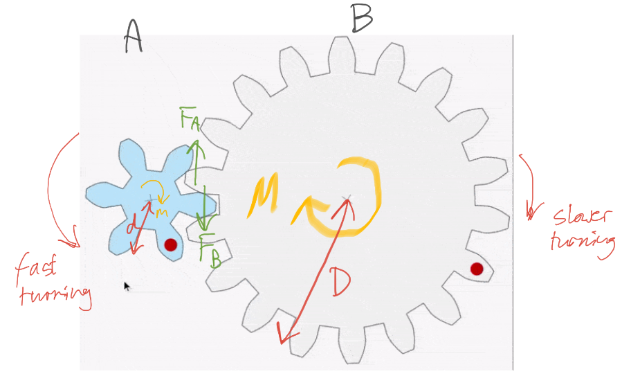
The driving gear (coloured blue) is smaller and has 6 teeth compared with the large gear’s 18 teeth. This is called a reduction gear arrangement.
A reduction gear arrangement does two things:
It slows down the speed of rotation. You may notice that the large gear turns only one for each three turns of the small gear.
The larger gear exerts a larger moment than the smaller gear. This is because the distance from the centre to the edge is larger for the grey gear.
The blue gear A exerts a force FA on gear B. By Newton’s Third Law, gear B exerts an equal but opposite force FB on gear A. Let’s take the magnitude of both forces to be F.
The anticlockwise moment exerted by gear A is given by m = F x d. The clockwise moment exerted by gear B is given by M=F x D. Since D > d then M > m.
A reduction gear arrangement is typically used in devices like an electric screwdriver. The electric motor in the device produces only a small rotational moment m but a large moment M is needed to turn the screws. The reduction gear produces the large moment M required.
Part 2: The overdrive arrangement
What happens when the driver gear is larger and has a greater number of teeth than the driven gear? This is called an overdrive arrangement.
The example we are going to look at is the arrangement of gears on a bicycle.
Here the driver gear (on the left) is linked via a chain to the smaller driven gear on the right. This means that the anticlockwise moment of the first gear is transmitted directly to the second gear as an anticlockwise moment. That is to say, the direction of the moment is not reversed as it is when the two gears are directly linked by interlocking teeth.
In the example shown, the big gear A turns only once for each four turns completed by the smaller gear B. Let’s assume that gear A exerts a force F on the chain so that the chain exerts an identical force F on gear B. Since D > d, this means that M > m so that the arrangement works as a distance multiplier rather than a force multiplier. This is, of course, excellent if we are riding at speed along a horizontal road. However, if we encounter an upward incline we may wish to — using the gear changing arrangement on the bike — swap the small gear B with one with a larger value of d. This would have the happy effect of increasing the magnitude of m so as to make it slightly easier to pedal uphill.
You can get encouragingly accurate values for the speed of sound in the school laboratory using a tape measure and two smartphones (or tablets) running the Phyphox app.
Phyphox (pronounced FEE-fox) is an award-winning free app that was developed by physicists at Aachen University who wanted to give users direct access to the many sensors (e.g. accelerometers and magnetometers) which are standard features on many smartphones. In effect, it turns even the humblest smartphone or tablet into a multifunctional measuring instrument comparable to one of Star Trek’s famous ‘tricorders’.
To measure the speed of sound, we need two smartphones or tablets running Phyphox. We will be using the ‘Acoustic Stopwatch’ which measures the time between two acoustic events.
Phyphox main screen
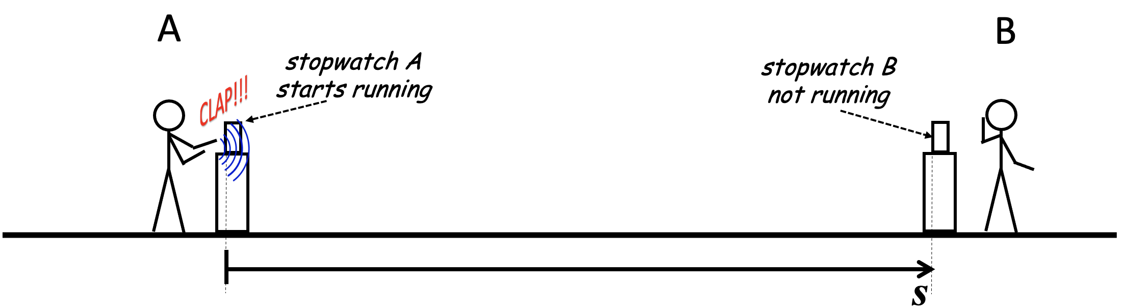
Step 1: Place two devices a measured distance s apart. Typically about 2 or 3 m should be OK otherwise the sound made by A will not be loud enough to control stopwatch B — this can be established through trial and error and depends on many factors including the background noise level.
Step 2: Person A makes a loud sound (a clap or a single syllable shout like ‘Hey!’ is good).
Step 3: Person B and stopwatch B wait for sound created by A to reach them.Step 4: The sound reaches stopwatch B and starts it running and B hears the sound.
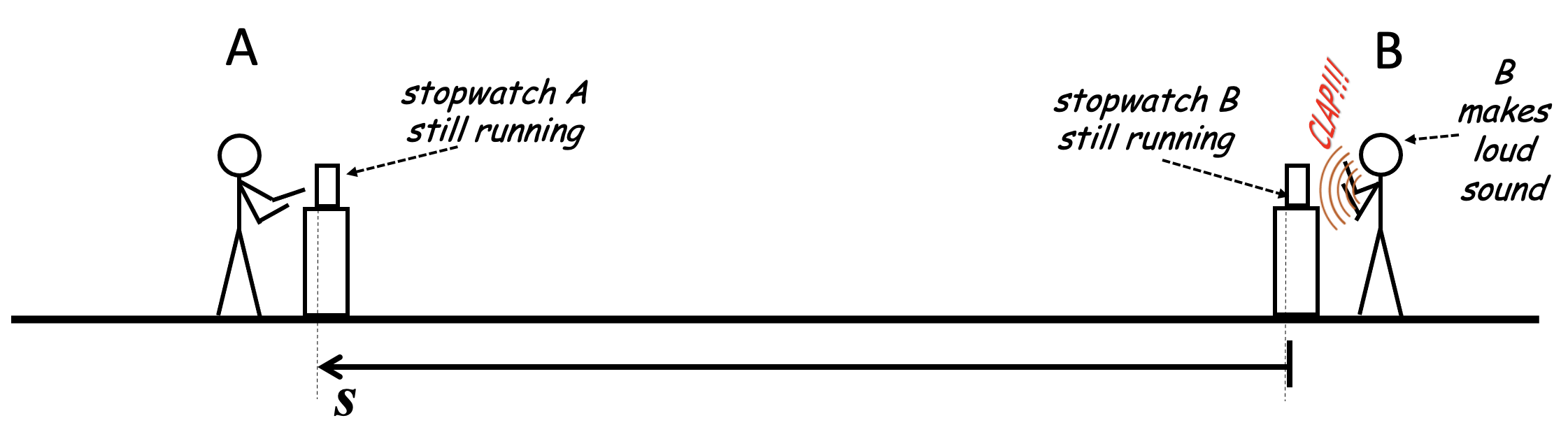
Step 5: B makes a loud sound in response.
Step 6: The loud sound made by B reaches stopwatch B and makes it stop. Let’s call the time displayed tB. This measures the delay between the sound from A reaching stopwatch B and B reacting to the sound and stopping the clock. It includes the time taken for the initial sound travelling from the device to B, B’s reaction time, and the time taken for the sound made by B to travel to stopwatch B. B does not have to be particularly ‘quick off the mark’ to respond to A’s sound — although the shorter the time then the less likely it is then a background noise will interrupt the experiment.
Step 7: The sound made by B travels toward stopwatch A.
Step 8: The sound made by B reaches stopwatch A and makes it stop. Let’s call the time recorded on stopwatch A tA.
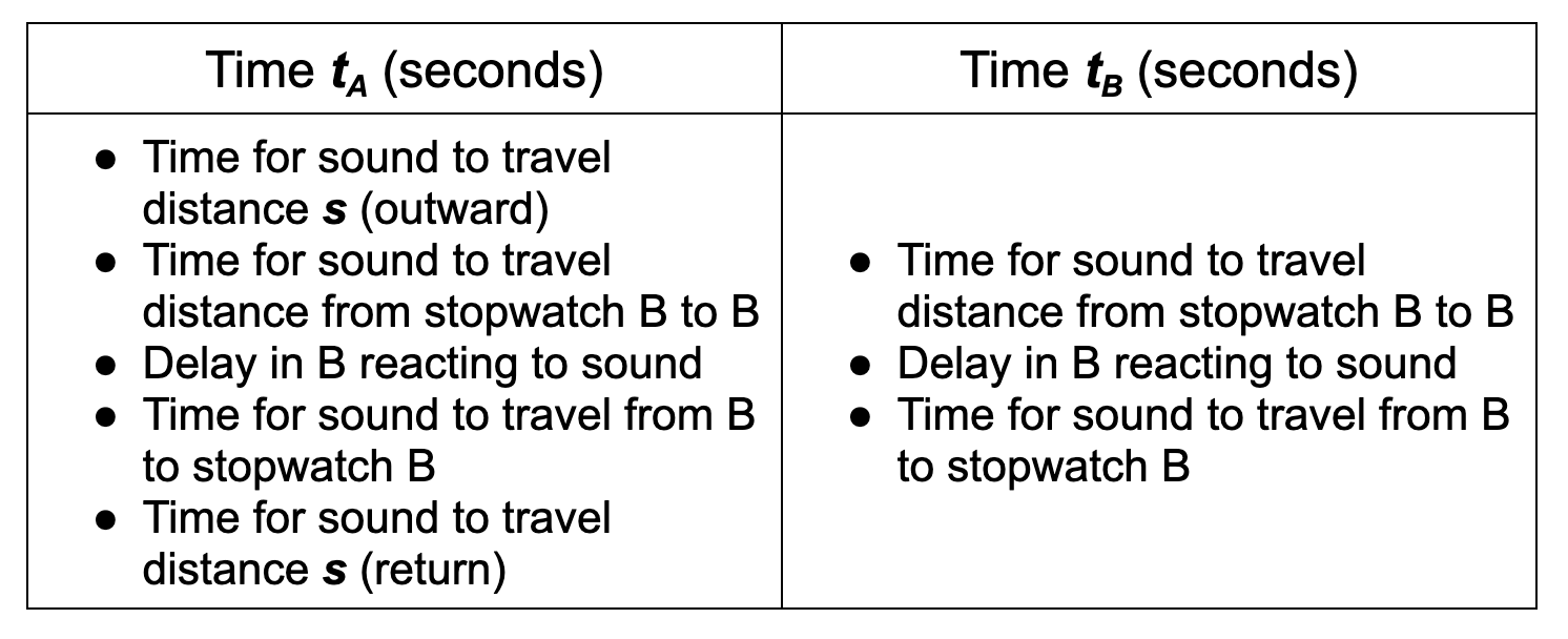
If we break down the events included in tA and tB, we find that tA is always larger than tB:
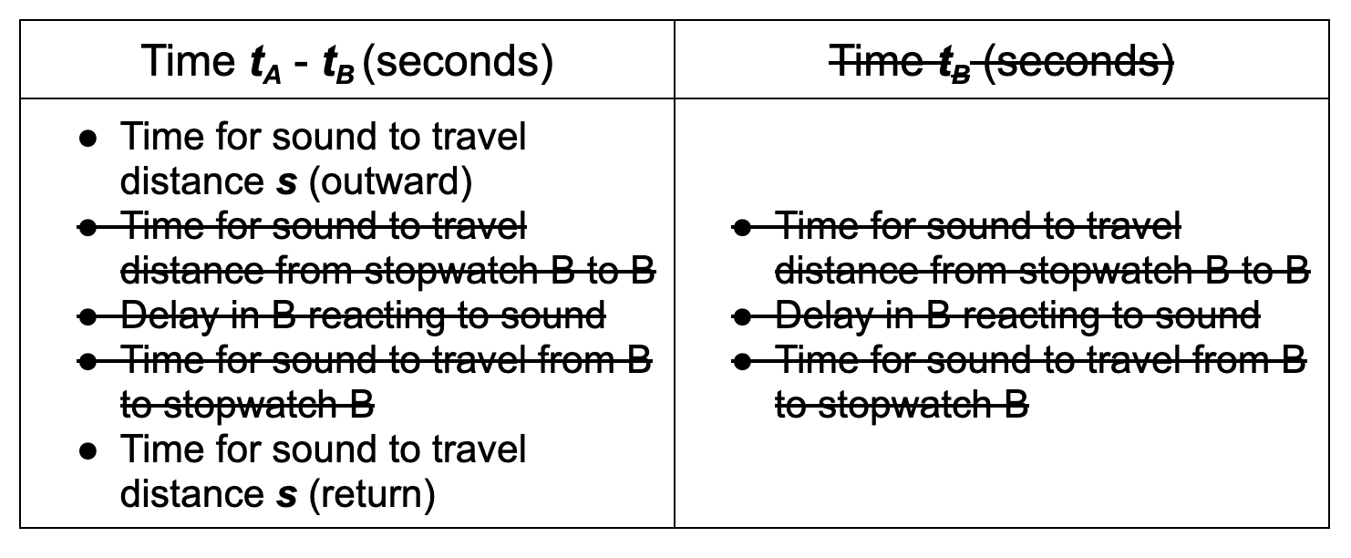
If we subtract tA – tB we find that this is the time it takes sound to travel a distance of 2s.
Step 9: We can therefore use this formula to find the v the speed of sound.
We have found that this method works well giving mean values of about 350 m/s for the speed of sound (which will vary with air temperature). This video models the method.
And so we have a reasonably practicable method of measuring the speed of that doesn’t involve complex equipment that is unfamiliar to most students; or a method that involves finding a large and featureless wall that produces a detectable echo when a loud sound is made from a point several metres in front of it.
I don’t know about you, but as a physics teacher, I feel cheated. If it doesn’t involve a double beam oscilloscope, a signal generator, two microphones and two power amplifiers then I simply don’t want to know about it . . .
The Rite of AshkEnte, quite simply, summons and binds Death. Students of the occult will be aware that it can be performed with a simple incantation, three small bits of wood and 4cc of mouse blood, but no wizard worth his pointy hat would dream of doing anything so unimpressive; they knew in their hearts that if a spell didn’t involve big yellow candles, lots of rare incense, circles drawn on the floor with eight different colours of chalk and a few cauldrons around the place then it simply wasn’t worth contemplating.
‘Transformers’ is one of the trickier topics to teach for GCSE Physics and GCSE Combined Science.
I am not going to dive into the scientific principles underlying electromagnetic induction here (although you could read this post if you wanted to), but just give a brief overview suitable for a GCSE-level understanding of:
The basic principle of a transformer; and
How step down and step up transformers work.
One of the PowerPoints I have used for teaching transformers is here. This is best viewed in presenter mode to access the animations.
The basic principle of a transformer
A GIF showing the basic principle of a transformer. (BTW This can be copied and pasted into a presentation if you wish,)
The primary and secondary coils of a transformer are electrically isolated from each other. There is no charge flow between them.
The coils are also electrically isolated from the core that links them. The material of the core — iron — is chosen not for its electrical properties but rather for its magnetic properties. Iron is roughly 100 times more permeable (or transparent) to magnetic fields than air.
The coils of a transformer are linked, but they are linked magnetically rather than electrically. This is most noticeable when alternating current is supplied to the primary coil (green on the diagram above).
The current flowing in the primary coil sets up a magnetic field as shown by the purple lines on the diagram. Since the current is an alternating current it periodically changes size and direction 50 times per second (in the UK at least; other countries may use different frequencies). This means that the magnetic field also changes size and direction at a frequency of 50 hertz.
The magnetic field lines from the primary coil periodically intersect the secondary coil (red on the diagram). This changes the magnetic flux through the secondary coil and produces an alternating potential difference across its ends. This effect is called electromagnetic induction and was discovered by Michael Faraday in 1831.
Energy is transmitted — magnetically, not electrically — from the primary coil to the secondary coil.
As a matter of fact, a transformer core is carefully engineered so to limit the flow of electrical current. The changing magnetic field can induce circular patterns of current flow (called eddy currents) within the material of the core. These are usually bad news as they heat up the core and make the transformer less efficient. (Eddy currents are good news, however, when they are created in the base of a saucepan on an induction hob.)
Stepping Down
One of the great things about transformers is that they can transform any alternating potential difference. For example, a step down transformer will reduce the potential difference.
A GIF showing the basic principle of a step down transformer. (BTW This can be copied and pasted into a presentation if you wish,)
The secondary coil (red) has half the number of turns of the primary coil (green). This halves the amount of electromagnetic induction happening which produces a reduced output voltage: you put in 10 V but get out 5 V.
And why would you want to do this? One reason might be to step down the potential difference to a safer level. The output potential difference can be adjusted by altering the ratio of secondary turns to primary turns.
One other reason might be to boost the current output: for a perfectly efficient transformer (a reasonable assumption as their efficiencies are typically 90% or better) the output power will equal the input power. We can calculate this using the familiar P=VI formula (you can call this the ‘pervy equation’ if you wish to make it more memorable for your students).
Thus: Vp Ip = Vs Is so if Vs is reduced then Is must be increased. This is a consequence of the Principle of Conservation of Energy.
Stepping up
A GIF showing the basic principle of a step up transformer. (BTW This can be copied and pasted into a presentation if you wish,)
There are more turns on the secondary coil (red) than the primary (green) for a step up transformer. This means that there is an increased amount of electromagnetic induction at the secondary leading to an increased output potential difference.
Remember that the universe rarely gives us something for nothing as a result of that damned inconvenient Principle of Conservation of Energy. Since Vp Ip = Vs Is so if the output Vs is increased then Is must be reduced.
If the potential difference is stepped up then the current is stepped down, and vice versa.
Last nail in the coffin of the formula triangle…
Although many have tried, you cannot construct a formula triangle to help students with transformer calculations.
Now is your chance to introduce students to a far more sensible and versatile procedure like FIFA (more details on the PowerPoint linked to above)
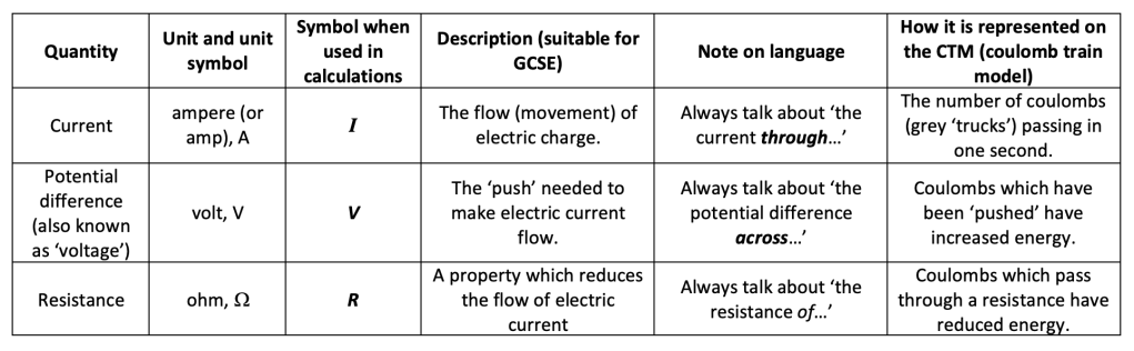
In this post, we are going to look at series circuits using the Coulomb Train Model.
The Coulomb Train Model (CTM) is a helpful model for both explaining and predicting the behaviour of real electric circuits which I think is useful for KS3 and KS4 students.
Without further ado, here is a a summary.
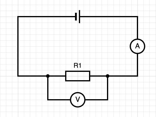
A circuit with one resistor
Let’s look at a very simple circuit to begin with:
This can be represented on the CTM like this:
The ammeter counts 5 coulombs passing every 10 seconds, so the current I = charge flow Q / time t = 5 coulombs / 10 seconds = 0.5 amperes.
We assume that the cell has a potential difference of 1.5 V so there is a potential difference of 1.5 V across the resistor R1 (that is to say, each coulomb loses 1.5 J of energy as it passes through R1).
The resistor R1 = potential difference V / current I = 1.5 / 0.5 = 3.0 ohms.
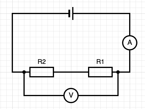
A circuit with two resistors in series
Now let’s add a second identical resistor R2 into the circuit.
This can be shown using the CTM like this:
Notice that the current in this example is smaller than in the first circuit; that is to say, fewer coulombs go through the ammeter in the same time. This is because we have added a second resistor and remember that resistance is a property that reduces the current. (Try and avoid talking about a high resistance ‘slowing down’ the current because in many instances such as two conductors in parallel a high current can be modelled with no change in the speed of the coulombs.)
Notice also that the voltmeter is making identical measurements on both the circuit diagram and the CTM animation. It is measuring the total energy change of the coulombs as they pass through both R1 and R2.
The current I = charge flow Q / time t = 5 coulombs / 20 seconds = 0.25 amps. This is half the value of the current in the first circuit.
We have an identical cell of potential difference 1.5 V the voltmeter would measure 1.5 V. We can calculate the total resistance using R = V / I = 1.5 / 0.25 = 6.0 ohms.
This is to be expected since the total resistance R = R1 + R2 and R1 = 3.0 ohms and R2 = 3.0 ohms.
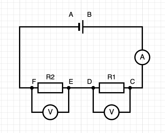
Looking at the resistors individually
The above circuit can be represented using the CTM as follows:
Between A and B, the coulombs are each gaining 1.5 joules since the cell has a potential difference of 1.5 V. (Remember that V = E energy transferred (in joules) / Q charge flow (in coulombs.)
Between B and C the coulombs lose no energy; that is to say, we are assuming that the connecting wires have negligible resistance.
Between C and D the coulombs lose some energy. We can use the familar V = I x R to calculate how much energy is lost from each coulomb, since we know that R1 is 3.0 ohms and I is 0.25 amperes (see previous section).
V = I x R = 0.25 x 3.0 = 0.75 volts.
That is to say, 0.75 joules are removed from each coulomb as they pass through R1 which means that (since 1.5 joules were added to each coulomb by the cell) that 0.75 joules are left in each coulomb.
The coulombs do not lose any energy travelling between D and E because, again, we are assuming negligible resistance in the connecting wire.
0.75 joules is removed from each coulomb between E and F making the potential difference across R2 to be 0.75 volts.
Thus we find that the familiar V = V1 + V2 is a direct consequence of the Principle of Conservation of Energy.
FAQ: ‘How do the coulombs know to drop off only half their energy in R1?’
Simple answer: they don’t.
This may be a valid objection for some donation models of electric circuits (such as the pizza delivery van model) but it doesn’t apply to the CTM because it is a continuous chain model (with the caveat that the CTM applies only to ‘steady state’ circuits where the current is constant).
Let’s look at a numerical argument to support this:
The magnitude of the current is controlled by only two factors: the potential difference of the cell and the total resistance of the circuit.
In other words, if we increased the value of R1 to (say) 4 ohms and reduced the value of R2 to 2 ohms so that the total resistance was still 6 ohms, the current would still be 0.25 amps.
However, in this case the energy dissipated by each coulomb passing through R1 would V = I x R = 0.25 x 4 = 1 volt (or 1 joule per coulomb) and similarly the potential difference across R2 would now be 0.5 volts.
The coulombs do not ‘know’ to drop off 1 joule at R1 and 0.5 joules at R2: rather, it is a purely mechanical interaction between the moving coulombs and each resistor.
R1 has a bigger proportion of the total resistance of the circuit than R2 so it seems self-evident (at least to me) that the coulombs will lose a larger proportion of their total energy passing through R1.
A similar analysis would apply if we made R2 = 4 ohms and R1 = 2 ohms: the coulombs would now lose 0.5 joules passing through R1 and 1 joule passing through R2.
Thus, we see that the current in a series circuit is affected by the ‘global’ or ‘whole circuit’ properties such as the potential difference of the cell and the total resistance of the circuit. The CTM models this property of real circuits by being a continuous chain of mechanically-linked ‘trucks’ so that a change in any one part of the circuit affects the movement of all the coulombs.
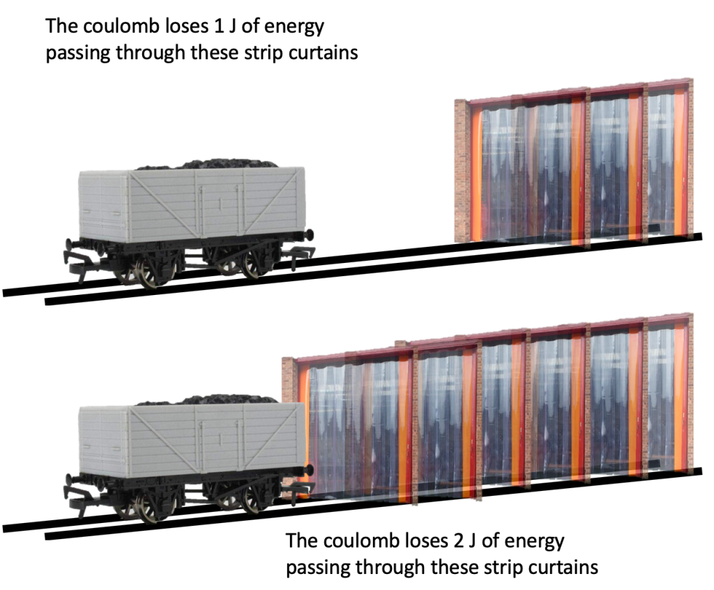
However, the proportion of the energy lost by a coulomb travelling through one part of the circuit is affected — not by ‘magic’ or a weird form of ‘coulomb telepathy’ — but only by the ‘local’ properties of that section of the circuit i.e. the electrical resistance of that section.
The CTM analogue of a low resistance section of a circuit (top) and a high resistance section of a circuit (bottom)
(PS You can read more about the CTM and potential divider circuits here.)
Afterword
You may be relieved to hear that this is the last post in my series on ‘The CTM revisited’. My thanks to the readers who have stayed with me through the series (!)
I will close by saying that I have appreciated both the expressions of enthusiasm about CTM and the thoughtful criticisms of it.
The Coulomb Train Model (CTM) is a helpful model for both explaining and predicting the behaviour of real electric circuits which I think is useful for KS3 and KS4 students.
Without further ado, here is a a summary.
This is part 4 of a continuing series. (Click to read Part 1, Part 2 or Part 3.)
The ‘Parallel First’ Heresy
I advocate teaching parallel circuits before teaching series circuits. This, I must confess, sometimes makes me feel like Captain Rum from Blackadder Two:
The main reason for this is that parallel circuits are conceptually easier to analyse than series circuits because you can do so using a relatively naive notion of ‘flow’ and gives students an opportunity to explore and apply the recently-introduced concept of ‘flow of charge’ in a straightforward context.
Redish and Kuo (2015: 584) argue that ‘flow’ is an example of embodiedcognition in the sense that its meaning is grounded in physical experience:
The thesis of embodied cognition states that ultimately our conceptual system grounded in our interaction with the physical world: How we construe even highly abstract meaning is constrained by and is often derived from our very concrete experiences in the physical world.
Redish and Kuo (2015: 569)
As an aside, I would mention that Redish and Kuo (2015) is an enduringly fascinating paper with a wealth of insights for any teacher of physics and I would strongly recommend that everyone reads it (see link in the Reference section).
Let’s Go Parallel First — but not yet
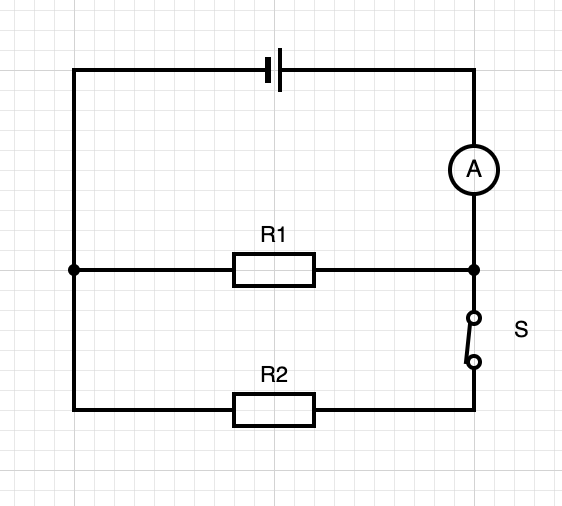
Let’s start with a very simple circuit.
This is not a parallel circuit (yet) because switch S is open. Resistors R1 and R2 are identical.
This can be represented on the coulomb train model like this:
Five coulombs pass through the ammeter in 20 seconds so the current I = Q/t = 5/20 = 0.25 amperes.
Let’s assume we have a 1.5 V cell so 1.5 joules of energy are added to each coulomb as they pass through the cell. Let’s also assume that we have negligible resistance in the cell and the connecting wires so 1.5 joules of energy will be removed from each coulomb as they pass through the resistor. The voltmeter as shown will read 1.5 volts.
The resistance of the resistor R1 is R=V/I = 1.5/0.25 = 6.0 ohms.
Let’s Go Parallel First — for real this time.
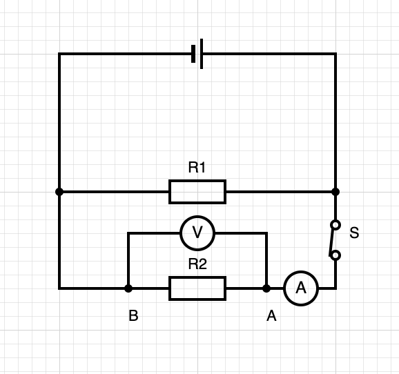
Now let’s close switch S.
This is example of changing an example by continuous conversion which removes the need for multiple ammeters in the circuit. The changed circuit can be represented on the CTM as shown
Now, ten coulombs pass through the ammeter in twenty seconds so I = Q/t = 10/20 = 0.5 amperes (double the reading in the first circuit shown).
Questioning may be useful at this point to reinforce the ‘flow’ paradigm that we hope students will be using:
What will be the reading if the ammeter moved to a similar position on the other side? (0.5 amps since current is not ‘used up’.)
What would be the reading if the ammeter was placed just before resistor R1? (0.25 amps since only half the current goes through R1.)
To calculate the total resistance of the whole circuit we use R = V/I = 1.5/0.5 = 3.0 ohms– which is half of the value of the circuit with just R1. Adding resistors in parallel has the surprising result of reducing the total resistance of the circuit.
This is a concrete example which helps students understand the concept of resistance as a property which reduces current: the current is larger when a second resistor is added so the total resistance must be smaller. Students often struggle with the idea of inverse relationships (i.e. as x increases y decreases and vice versa) so this is a point well worth emphasising.
Potential Difference and Parallel Circuits (1)
Let’s expand on the primitive ‘flow’ model we have been using until now and adapt the circuit a little bit.
This can be represented on the CTM like this:
Each coulomb passing through R2 loses 1.5 joules of energy so the voltmeter would read 1.5 volts.
One other point worth making is that the resistance of R2 (and R1) individually is still R = V/I = 1.5/0.25 = 6.0 ohms: it is only the combined effect of R1 and R2 together in parallel that reduces the total resistance of the circuit.
Potential Difference and Parallel Circuits (2)
Let’s have one last look at a different aspect of this circuit.
This can be represented on the CTM like this:
Each coulomb passing through the cell from X to Y gains 1.5 joules of energy, so the voltmeter would read 1.5 volts.
However, since we have twice the number of coulombs passing through the cell as when switch S is open, then the cell has to load twice as many coulombs with 1.5 joules in the same time.
This means that, although the potential difference is still 1.5 volts, the cell is working twice as hard.
The result of this is that the cell’s chemical energy store will be depleted more quickly when switch S is closed: parallel circuits will make cells go ‘flat’ in a much shorter time compared with a similar series circuit.
Bulbs in parallel may shine brighter (at least in terms of total brightness rather than individual brightness) but they won’t burn for as long.
To some ways of thinking, a parallel circuit with two bulbs is very much like burning a candle at both ends…
More fun and high jinks with coulomb train model in the next instalment when we will look at series circuits.
‘FIFA’ in this context has nothing to do with football; rather, it is a mnemonic that helps KS3 and KS4 students from across the attainment range engage productively with calculation questions.
FIFA stands for:
Formula
Insert values
Fine-tune
Answer
From personal experience, I can say that FIFA has worked to boost physics outcomes in the schools I have worked in. What is especially gratifying, however, is that a number of fellow teaching professionals have been kind enough to share their experience of using it:
Framing FIFA as a modular approach
Straightforward calculation questions (typically 2 or 3 marks) can be ‘unlocked’ using the original FIFA approach. More challenging questions (typically 4 or 5 marks) can often be handled using the FIFA-one-two approach.
However, what about the most challenging 5 or 6 mark questions that are targeted at Grade 8/9? Can FIFA help in solving these?
I believe it can. But before we dive into that, let’s look at a more traditional, non-FIFA, algebraic approach.
A challenging freezing question: the traditional (non-FIFA) algebraic approach
Note: this is a ‘made up’ question written in the style of the GCSE exam.
A pdf of this question is here. A traditional algebraic approach to solving this problem would look like this:
This approach would be fine for confident students with high previous attainment in physics and mathematics. I will go further and say that it should be positively encouraged for students who possess — in Edward Gibbon’s words — that ‘happy disposition’:
But the power of instruction is seldom of much efficacy, except in those happy dispositions where it is almost superfluous.
Edward Gibbon, The Decline and Fall of the Roman Empire
But what about those students who are more akin to the rest of us, and for whom the ‘power of instruction’ is not a superfluity but rather a necessity on which they depend?
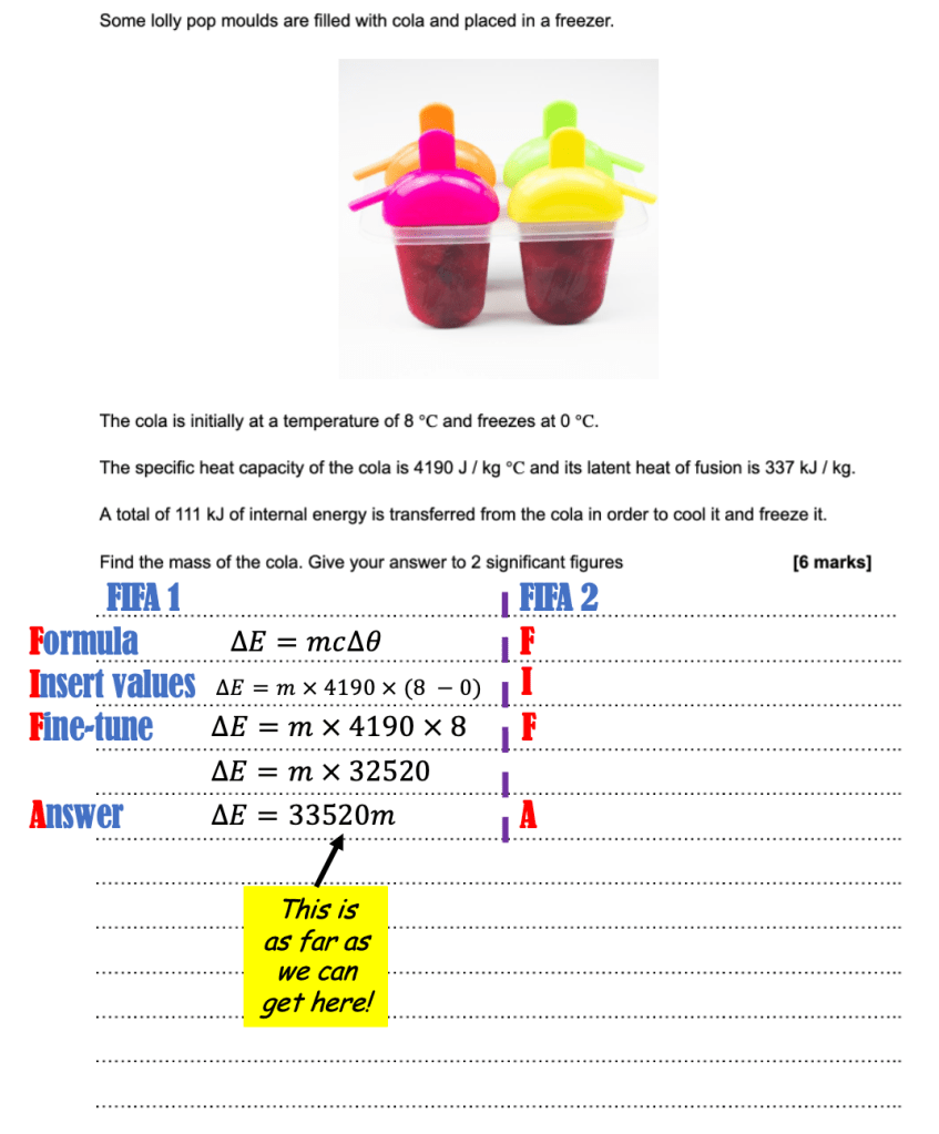
A challenging freezing question: the FIFA-1-2-3 approach
Since this question involves both cooling and freezing it seems reasonable to start with the specific heat capacity formula and then use the specific latent heat formula:
Cold-calling students and asking them: ‘What should we write in this box?’ is, surprisingly, an effective way of engaging the class in the process. It’s good to emphasise that we write in numbers for the the values we know from the question and symbols for the ones we don’t.It is important to model how to deal with values that we don’t know…This is far as we can get using the FIFA-one-two model….
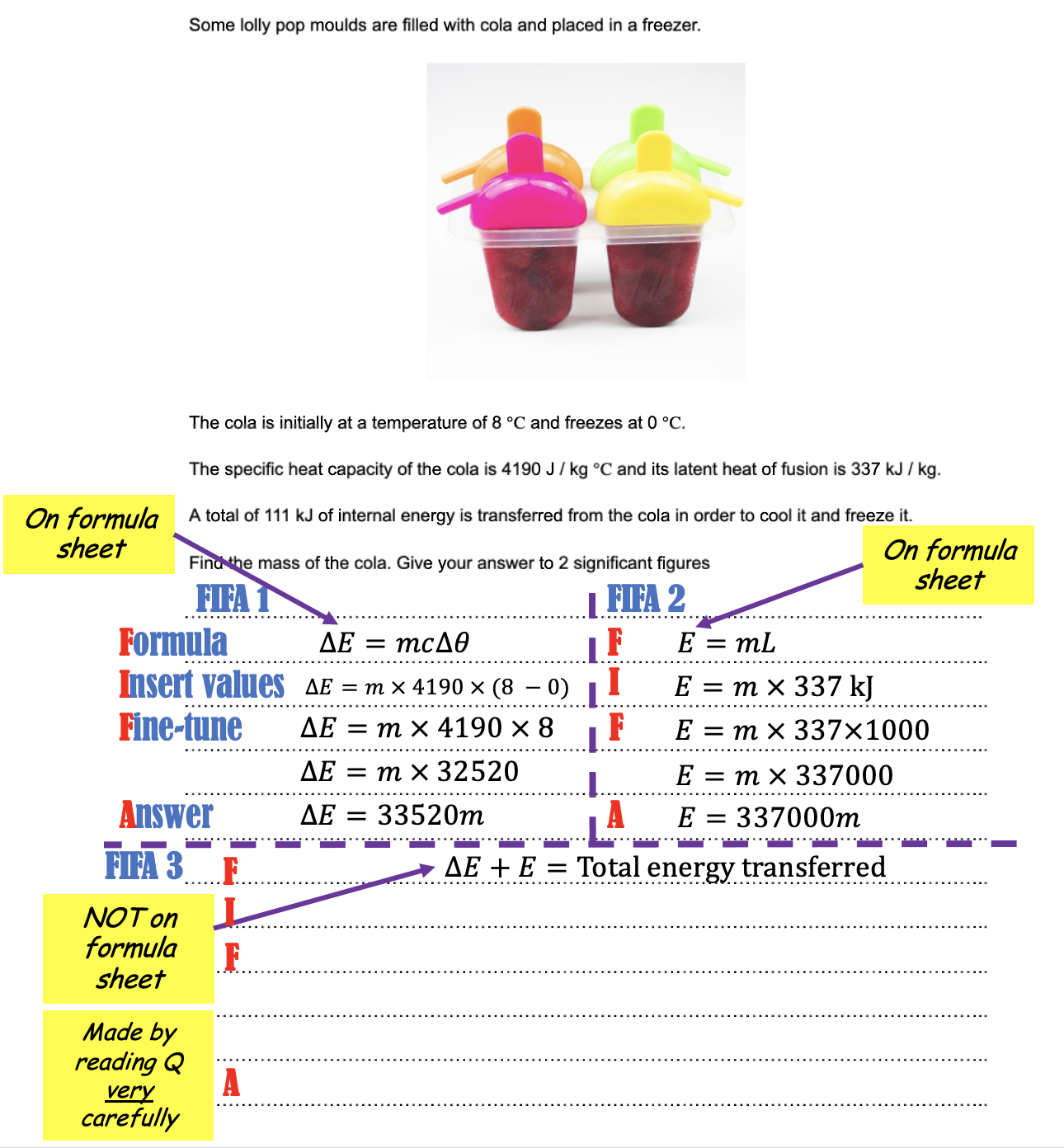
FIFA-one-two isn’t enough. We must resort to FIFA-1-2-3.
What is noteworthy here is that the third FIFA formula isn’t on the formula sheet and is not on the list of formulas that need to be memorised. Instead, it is made by the student based on their understanding of physics and a close reading of the question.
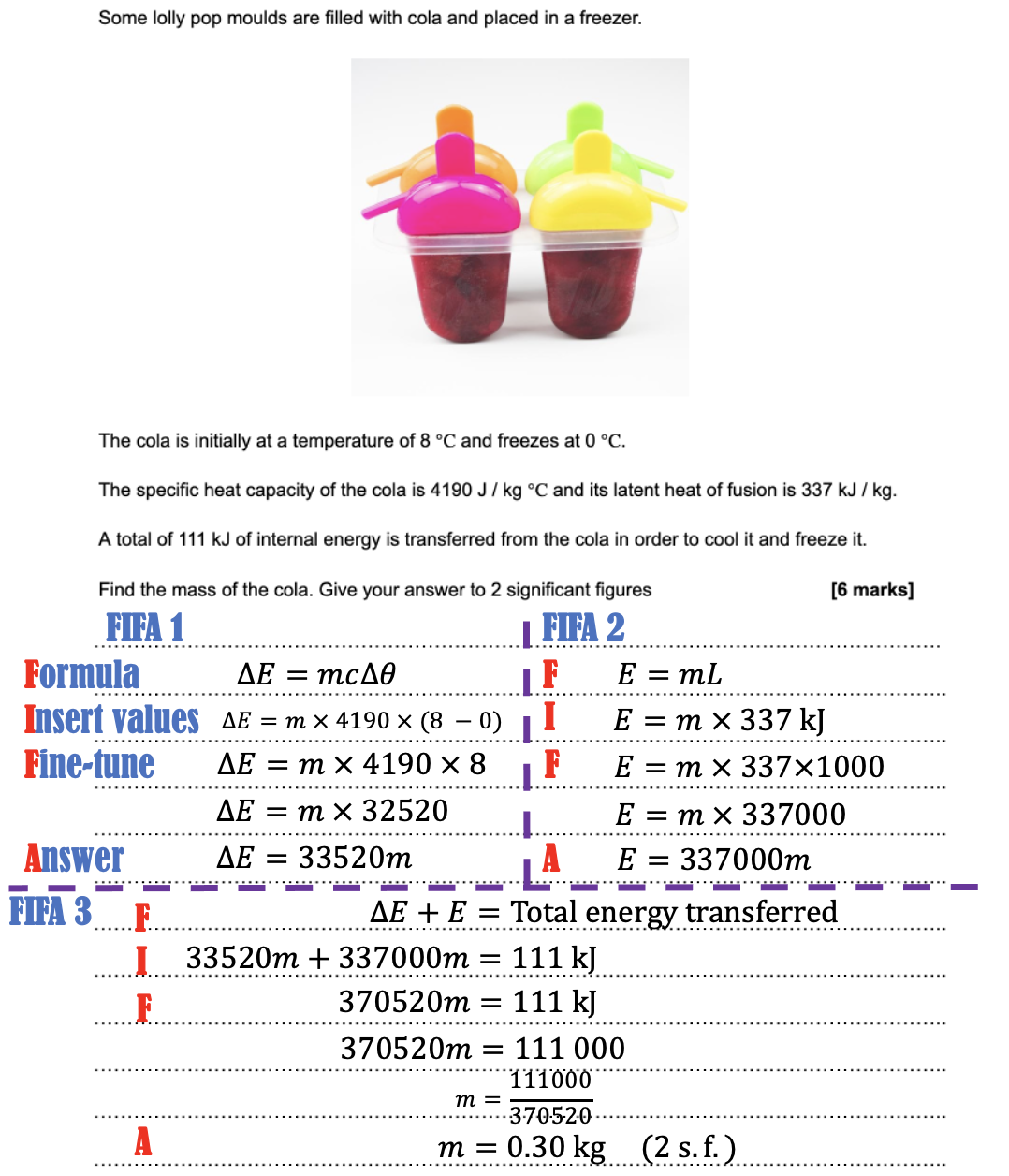
Challenging? Yes, undoubtedly. But students will have unlocked some marks (up to 4 out of 6 by my estimation).
FIFA isn’t a royal road to mathematical mastery (although it certainly is a better bet than the dreaded ‘formula triangle’ that I and many other have used in the past). FIFA is the scaffolding, not the finished product.
Genuine scientific understanding is the clock tower; FIFA is simply some temporary scaffolding that helps students get there.
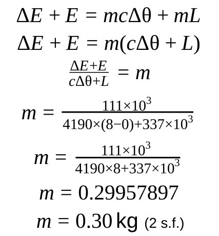
We complete the FIFA-1-2-3 process as follows:
Conclusion: FIFA fixes it
The FIFA-system was born of the despair engendered when you mark a set of mock exam papers and the majority of pages are blank: students had not even attempted the calculation skills.
In my experience, FIFA fixes that — students are much more willing to start a calculation question. And that means that, even when they cannot successfully navigate to a ‘full mark’ conclusion, they gain at least some marks, and and one does not have to be a particularly perceptive scholar of the human heart to understand that gaining ‘some marks‘ is more motivating than ‘no marks‘.
Update: Ed Southall makes a persuasive case against formula triangles in this 2016 article.