The worst circuit in the world

“The most miserable latch that’s ever been designed in the history of mankind or before.”

Astronaut Jack R. Lousma commenting on some equipment issues during the NASA Skylab 3 mission (July to September 1973), quoted in Cooper 1976: 41

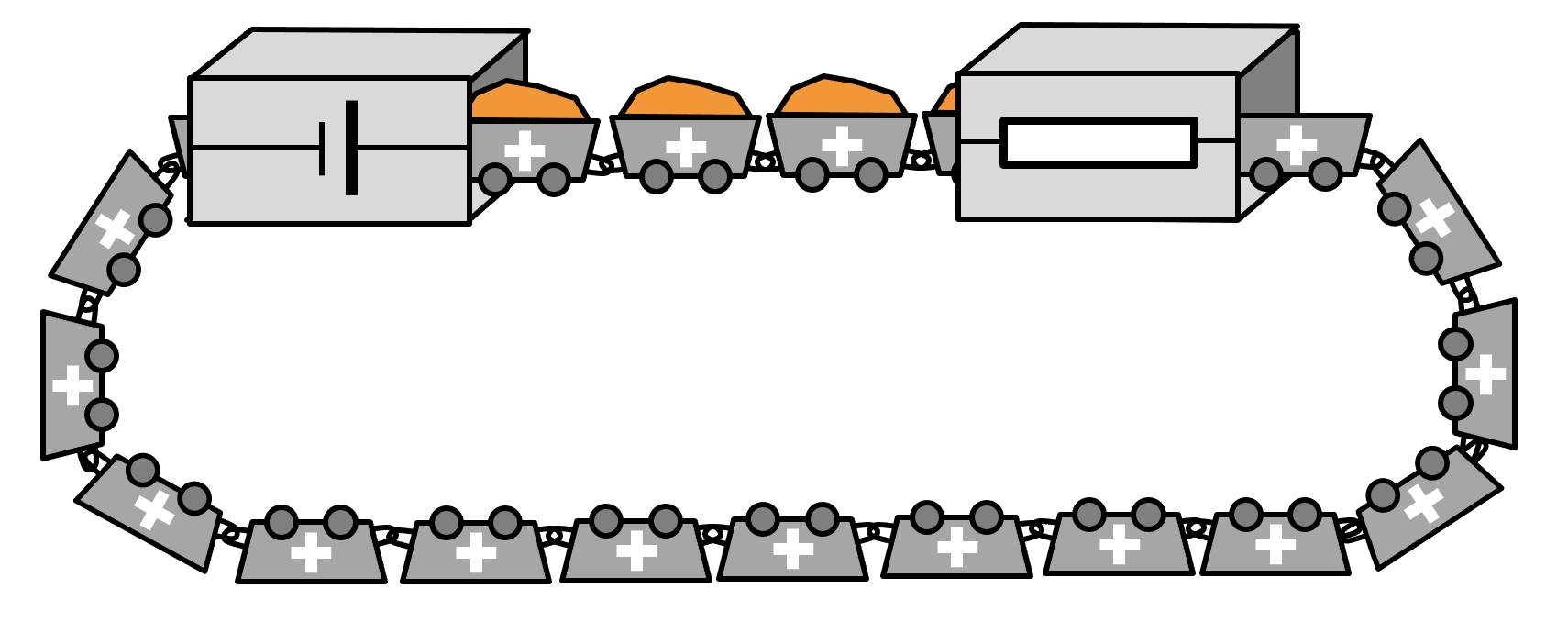
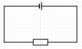
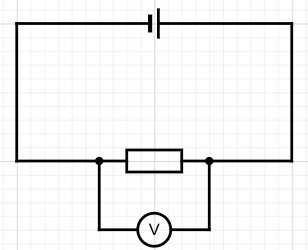
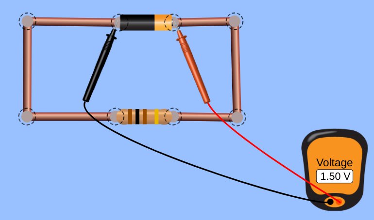
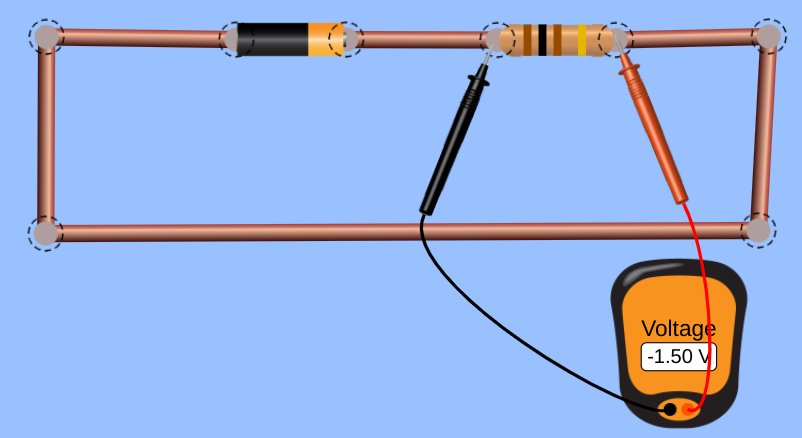
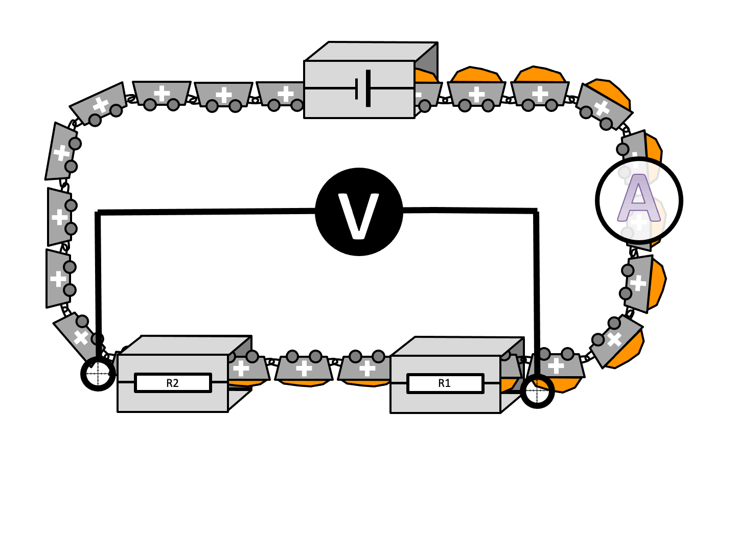
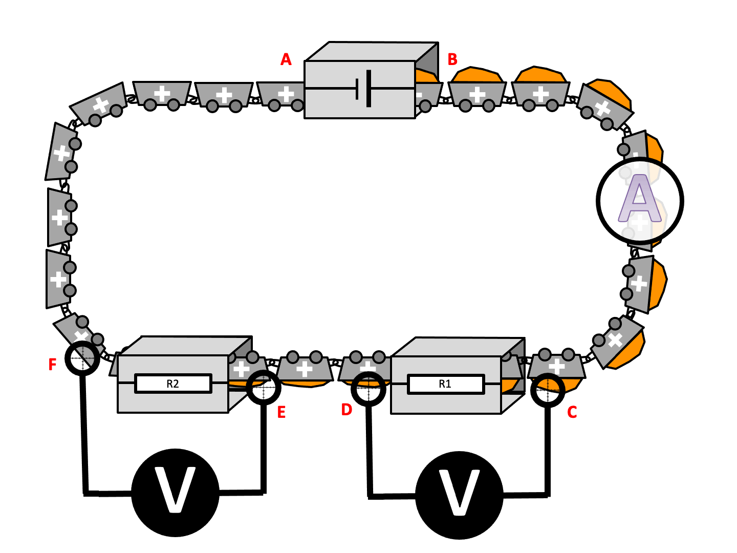
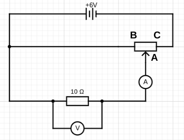
What does the worst circuit that’s ever been designed in the history of humankind or before look like? Without further ado, here it is:

‘But wait,’ I hear you say, ‘isn’t this the circuit intended for obtaining the data for plotting current-potential difference characteristic curves as recommended by the AQA exam board in their GCSE Physics and GCSE Combined Science specifications?’ (AQA 2018: 47)

Sadly, it is indeed.

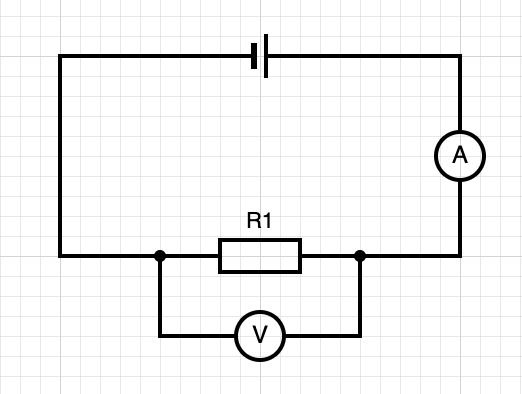
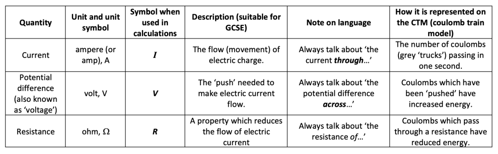
Why is ‘the standard test circuit’ a *bad* circuit?

The point of this required practical is to get several paired readings of potential difference across a component and the current through a component to enable us to plot a graph (aka ‘characteristic’) of current against potential difference. Ideally, we would like to start at 0.0 volts across the resistor and measure the current at (say) 1.0, 2.0, 3.0, 4.0, 5.0 and 6.0 volts. That is to say, we would like to treat the potential difference as the independent variable and adjust it in consistent, regular increments.

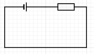
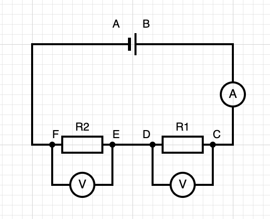
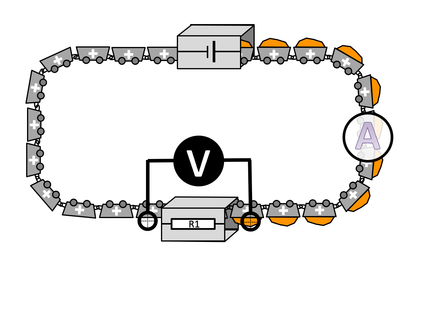
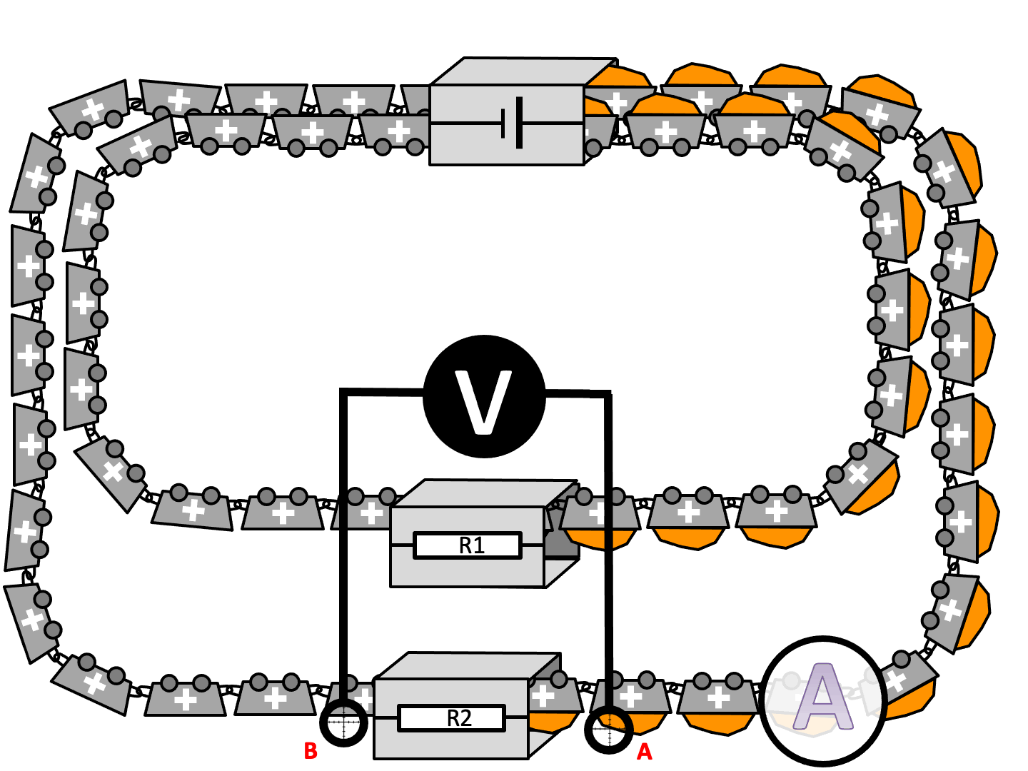
Now let’s say we use a typical school rheostat such as the one shown below as the variable resistor in series with the 10 ohm resistor. The two of them will behave as a potential divider circuit (see here and here for posts on this topic).

The resistance of the variable resistor can be varied between 0 and 16 ohms by moving the slider. When the slider is at A it will have the maximum resistance of 16 ohms and zero when it is at C, and in-between values at any other point.

A typical school rheostat. To use as a simple variable resistor, connect only terminals A and C into the circuit. (Please note: using terminals B and C will make it behave as a fixed resistor.)

When the slider is at C, the 10 ohm resistor gets the full potential difference from the supply and so the voltmeter will read 6.0 V and the ammeter will read (using I=V/R) 6.0 / 10 = 0.6 amps.

When the slider is at A, the total resistance of the circuit is 10 + 16 = 26 ohms so the ammeter reading (again using I=V/R) will be 6.0/26 = 0.23 amps. This means that the voltmeter reading (using V=IR) will be 0.23 x 10 = 2.3 volts.

This means that the circuit as presented will only allow us to obtain potential differences between a minimum of 2.3 V and a maximum of 6.0 V across the component by moving the slider between B and C, which is less than ideal.

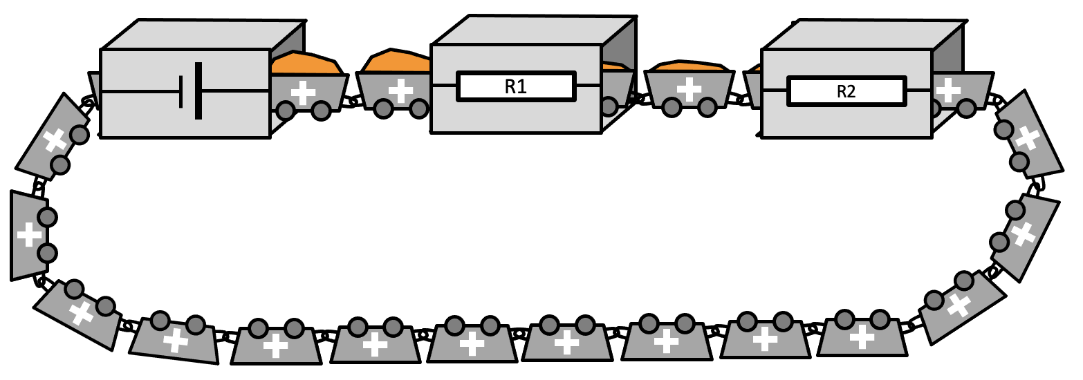
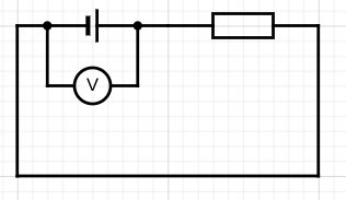
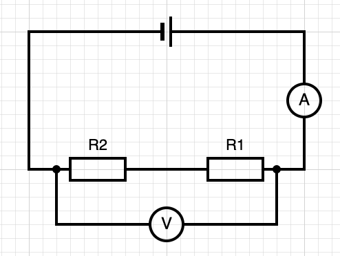
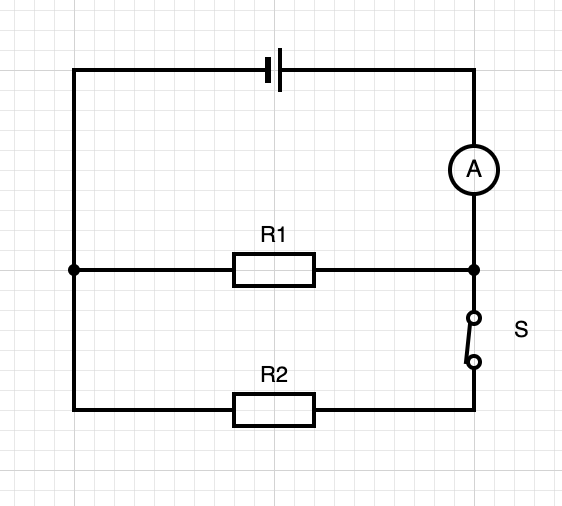
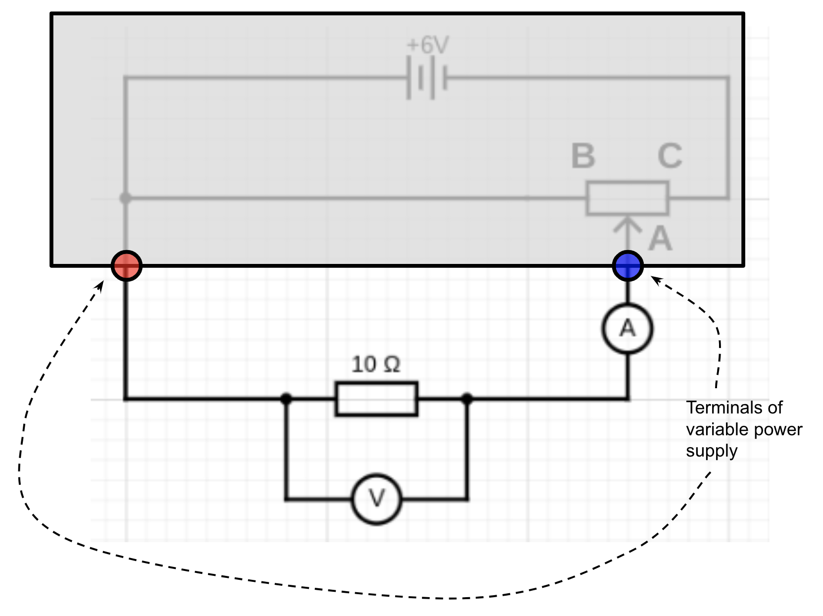
‘It is a far, far better circuit that I build than I have ever built before…’

It is a far, far better thing that I do, than I have ever done.

Charles Dickens, ‘A Tale of Two Cities’

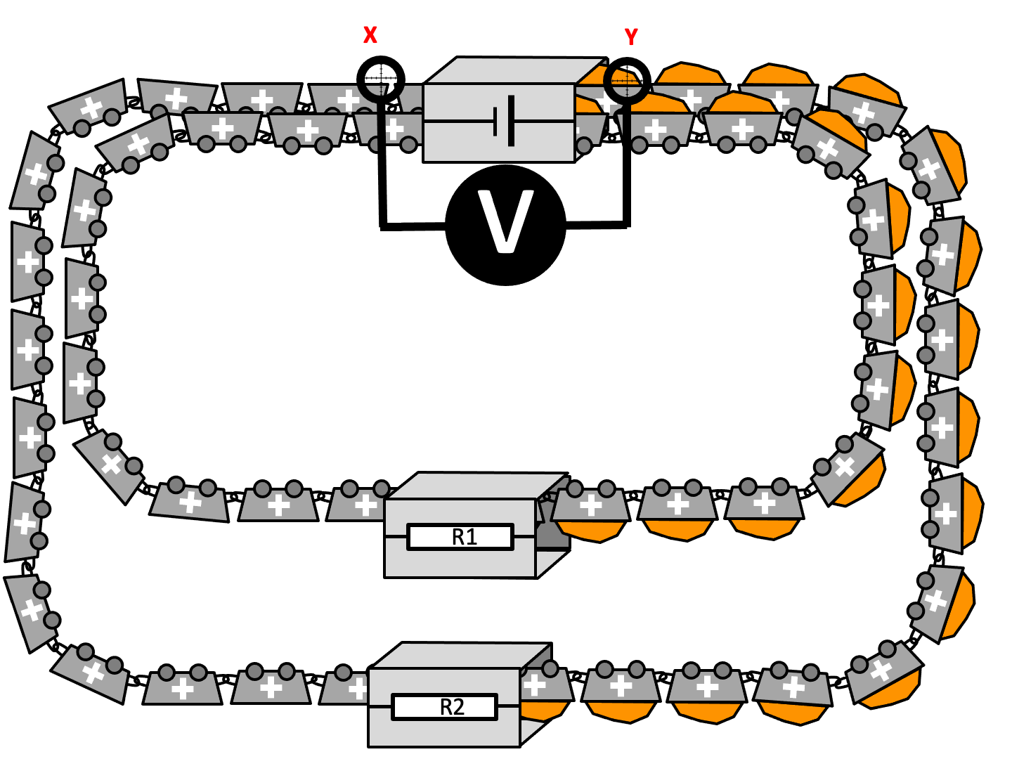
This circuit is a far better one for obtaining the data for a current-potential difference graph. This is because we can access the full 0.0 V to 6.0 V of the supply simply by adjusting the position of the rheostat slider. The rheostat is being used as a potential divider in this circuit rather than as a simple variable resistor.

When the slider is at B, the voltmeter will read 0.0 V and the current through the 10 ohm resistor will be 0.0 amps. A small movement of the slider from B towards C will increase the reading of the voltmeter to (say) 1.0 V and the ammeter would read 0.1 A. Further small movements of the slider will gradually increase the potential difference across the resistor until it reaches the full 6.0 V when the slider is at C.

A-level Physics students are expected to be able to use this circuit and enumerate its advantages over the ‘worst circuit in the world’.

And, to be fair, AQA do suggest a workaround that will allow GCSE student to side-step using ‘the worst circuit in the world’:

If a lab pack is used for the power supply this can remove the need for the rheostat as the potential difference can be varied directly. The voltage should not be allowed to get so high as to damage the components, check the rating of the components you plan to suggest your students use.

AQA 2018: 16
A ‘lab pack’ i.e. a power supply with a variable output potential difference

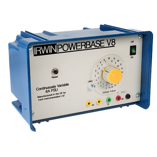
If this method is used, then in effect you would be using the ‘built in’ rheostat inside the power supply.

So why not use the superior potential divider circuit at GCSE?

The arguments in favour of using ‘the worst circuit in the world’ as opposed to the more fit for purpose potential divider circuit are:

  1. The ‘worst circuit in the world’ is (arguably) conceptually easier than the potential divider circuit, especially if students have not studied series and parallel circuit before. This allows more freedom in sequencing when IV characteristics are taught.
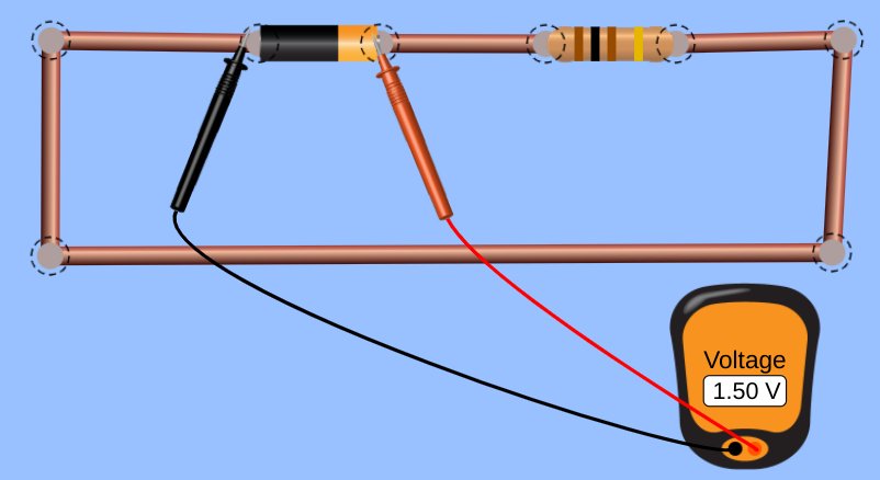
  2. A fuller range of potential differences can be accessed even using the ‘worst circuit in the world’ if the maximum value of the variable resistor is much larger than the resistance of the component. For example, if we used a 0 – 1 kilo-ohm variable resistor in series with the 10 ohm resistor then very fine adjustments of the variable resistor would allow a suitable range of potential difference to be applied across the component.
  3. Students are often asked direct questions about the ‘worst circuit in world’.
Question from AQA Paper 1 (2021) where students who have used ‘the worst circuit in the world’ for their investigation would (imo) have an advantage over those that have not.

In the next post, I will outline how I introduce and teach this required practical — using, to my shame, ‘the worst circuit in the world’ — and also supply some useful resources.

You can read part 2 here.

REFERENCES

AQA (2018). Practical Handbook: GCSE Physics. Retrieved from https://filestore.aqa.org.uk/resources/physics/AQA-8463-PRACTICALS-HB.PDF on 7/5/23

Cooper, H. S. F. (1976). A House In Space. New York: Bantam Books

Modelling Electrical Power Equations using the CTM

The Coulomb Train Model (CTM) is a straightforward, easily pictured representation that helps novice learners develop an initial “sense of mechanism” about how electric circuits work. You can read about it here and here (and, to some extent, track its development over time).

In this post, however, I want to focus on how effective the CTM is in helping students understand the energy and power formulas associated with electric circuits: notably E = QV, P = IV and P=I2R.

E=QV and the CTM

An animated version of the Coulomb Train Model

The E in E=QV stands for the energy transferred to the bulb by the electric current (in joules, J). The Q is the charge flow in coulombs, C. The V is the potential difference across the resistor in volts, V.

Using the Coulomb Train Model:

  • Each grey truck passing through the bulb represents one coulomb of charge flow. Q is therefore the number of grey trucks passing through the bulb in a certain time t. (We won’t specify what that time t is now but we will return to it shortly.)
  • The potential difference V is the energy transferred out of each coulomb as they pass through the bulb. If one joule (represented by the orange stuff in the truck) is transferred from each coulomb then the potential difference is one volt. If two joules then the potential difference is two volts, and so on.

How can we increase the energy transferred into the bulb? There are two ways:

  1. Increase the total number of coulombs passing through the bulb. That is to say, increasing Q. We could do this by (a) waiting a longer time so that more coulombs pass through the bulb; or (b) increasing the current so that more coulombs pass through each second.
  2. Increase the energy transferred from each coulomb into the bulb. That is to say, increasing V. We could do this by increasing the potential difference of the cell so that each coulomb is loaded up with more energy.
Hewitt representation of changing the values of Q and V while keeping the other fixed

Or, of course, we could increase the values of Q and V simultaneously.

Hewitt representation of increasing Q and V simultaneously

All you need is E = Q V

In other words, the energy transferred per second (or the power P in watts, W) is equal to the product of the current I in amperes (or coulombs per second) and the potential difference V in volts, V.

A higher current will increase the power transferred to the bulb: more coulombs will pass through the bulb per second so more energy is transferred to the bulb each second. This can be modelled using the Coulomb Train Model as shown:

Using the CTM to show the relationship between current I and power P

Increasing the potential difference V (i.e. the energy carried by each coulomb) would also increase P.

Deriving P=I2R from P=IV

If we start with P=IV but remember that V=IR then P=I(IR) so P=I2R.

This can be represented on the Coulomb Train Model like this:

We can increase the power transferred to the resistor by:

  • Increasing the value of the resistor (and keeping I constant, which implies that V would have to be increased). Doubling the value of R would double the value of P.
  • Increasing the value of I. However, since the formula includes I squared then this would have a disproportionate effect on P. For example, if I was doubled then P would be quadrupled. A Hewitt representation can be useful for highlighting this to students; for example:
A Hewitt representation of the effect of doubling I on P

Linking the electrical power formulas

The electrical power equations when considered in isolation can seem random and unconnected. Making the links between them explicit can be not just a powerful aid to memory, but also hints at the power and coherence of that noble exploration of reality and possibility called physics.

Series and Parallel Circuits — an unhelpful dichotomy?

Anakin Skywalker and Obi Wan Kenobi discuss the possible unhelpfulness of the concept of ‘series circuits’ and ‘parallel circuits

Are physics teachers following the Way of the Sith? Are we all crossing over to the Dark Side when we talk about ‘series circuits’ and ‘parallel circuits’?

I think that, without meaning to, we may be presenting students with what amounts to a false dichotomy: that all circuits are either series circuits or parallel circuits.

Venn diagram showing the false dichotomy view of series and parallel circuits

The actual situation is more like this:

A Venn diagram showing a more nuanced and realistic view of series and parallel circuits

The confusion may stem from our usage of the word ‘circuit’: are we referring holistically to the entire assemblage of components (highlighted in red) or the individual ‘complete circuits’ (highlighted in green and blue)?

Will the actual ‘circuit’ please stand up? The red circuit is a hybrid circuit, the green circuit is a series circuit, and the blue circuit shows a single resistor in series or parallel with cell (depending on how you look at it)

How to avoid the false dichotomy

I think we should always refer to components in series or components in parallel rather than ‘series circuits’ or ‘parallel circuits’.

Teaching components in parallel using the ‘all-in-a-row’ circuit convention

I’ve written before about what I think is the confusing ‘hidden rotation’ present in normal circuit diagrams. I find redrawing circuit diagrams using the ‘all-in-a-row’ convention useful for explaining circuit behaviour. For simplicity, we’ll assume that all the resistors in the diagrams that follow have a resistance of one ohm.

This can be shown using the Coulomb Train Model like this (coulombs pictured as moving clockwise):

The reason the voltmeter across the cell reads +1.5 V is that energy is being transferred from the chemical energy store of the cell *into* the coulombs. The reason the voltmeter reads -1.5 V across the resistor is that energy is being transferred *from* the coulombs and into the thermal energy store of the resistor.

The current passing through the resistor using I = V/R = 1.5 V / 1 = 1.5 amperes.

Now let’s apply this convention when two resistors are in parallel.

This can be represented using the Coulomb Train Model like this:

I think it’s far clearer that ammeter W is measuring the total current in the circuit while X and Y are measuring the ‘part-current’ passing through R1 and R2 using this convention. (Note: we are assuming that each resistor has a resistance of one ohm.)

Each resistor has a potential difference of -1.5 V because 1.5 J of energy is being shifted from each coulomb as they pass through each resistor.

Also, it is clearer that the cell’s chemical energy store is being drained more quickly when there are two resistors in parallel: two coulombs have to be filled with 1.5 J of energy for each one coulomb in the single resistor circuit.

Thinking about current, the total current in the circuit is 3.0 amperes; so the resistance R = V / I = 1.5 / 3.0 = 0.5 ohms. So two resistors in parallel have a smaller resistance than a single resistor — this is a result that is well worth emphasising for students as so many of them find this completely counterintuitive!

Teaching components in series using the all-in-a-row convention

This circuit can be represented using the Coulomb Train Model like this:

The pattern of potential difference can be explained by looking at the orange ‘energy levels’ carried by each coulomb.

A current of one amp is one coulomb passing per second, so we can see that an ammeter reading would have the same value wherever the ammeter is placed in the circuit.

But look closely at R1: it only has 0.75 V of potential difference across. From I = V/R = 0.75 / 1 = 0.75 amperes.

This means that the total resistance of the circuit from R = V/I is, of course, 2 ohms.

Conclusion

I regret to say that I have probably been teaching ‘series circuits’ and ‘parallel circuits’ on autopilot for much of my career; the same may even be true of some readers of this blog(!)

The Coulomb Train Model has been considered in depth in previous blogs, but I think it’s a good model to encourage students to use their physical intuition (aka ’embodied cognition’) to understand electric circuits.

Whether you agree with the suggested outlines above or not, I hope that it has given you some fruitful food for thought.

Circuit Diagrams: Lost in Rotation…?

Is there a better way of presenting circuit diagrams to our students that will aid their understanding of potential difference?

I think that, possibly, there may be.

(Note: circuit diagrams produced using the excellent — and free! — web editor at https://www.circuit-diagram.org/.)

Old ways are the best ways…? (Spoiler: not always)

This is a very typical, conventional way of showing a simple circuit.

A simple circuit as usually presented

Now let’s measure the potential difference across the cell…

Measuring the potential difference across the cell

…and across the resistor.

Measuring the potential difference across the resistor

Using a standard school laboratory digital voltmeter and assuming a cell of emf 1.5 V and negligible internal resistance we would get a value of +1.5 volts for both positions.

Let me demonstrate this using the excellent — and free! — pHET circuit simulation website.

Indeed, one might argue with some very sound justification that both measurements are actually of the same potential difference and that there is no real difference between what we chose to call ‘the potential difference across the cell’ and ‘the potential difference across the resistor’.

Try another way…

But let’s consider drawing the circuit a different (but operationally identical) way:

The same circuit drawn ‘all-in-a-row’

What would happen if we measured the potential difference across the cell and the resistor as before…

This time, we get a reading (same assumptions as before) of [positive] +1.5 volts of potential difference for the potential difference across the cell and [negative] -1.5 volts for the potential difference across the resistor.

This, at least to me, is a far more conceptually helpful result for student understanding. It implies that the charge carriers are gaining energy as they pass through the cell, but losing energy as they pass through the resistor.

Using the Coulomb Train Model of circuit behaviour, this could be shown like this:

+1.5 V of potential difference represented using the Coulomb Train Model
-1.5 V of potential difference represented using the Coulomb Train Model. (Note: for a single resistor circuit, the emerging coulomb would have zero energy.)

We can, of course, obtain a similar result for the conventional layout, but only at the cost of ‘crossing the leads’ — a sin as heinous as ‘crossing the beams’ for some students (assuming they have seen the original Ghostbusters movie).

Crossing the leads on a voltmeter

A Hidden Rotation?

The argument I am making is that the conventional way of drawing simple circuits involves an implicit and hidden rotation of 180 degrees in terms of which end of the resistor is at a more positive potential.

A hidden rotation…?

Of course, experienced physics learners and instructors take this ‘hidden rotation’ in their stride. It is an example of the ‘curse of knowledge’: because we feel that it is not confusing we fail to anticipate that novice learners could find it confusing. Wherever possible, we should seek to make whatever is implicit as explicit as we can.

Conclusion

A translation is, of course, a sliding transformation, rather than a circumrotation. Hence, I had to dispense with this post’s original title of ‘Circuit Diagrams: Lost in Translation’.

However, I do genuinely feel that some students understanding of circuits could be inadvertently ‘lost in rotation’ as argued above.

I hope my fellow physics teachers try introducing potential difference using the ‘all-in-row’ orientation shown.

The all-in-a-row orientation for circuit diagrams to help student understanding of potential difference

I would be fascinated to know if they feel its a helpful contribition to their teaching repetoire!

Booklet for teaching the Coulomb Train Model

At the bottom of the post are some links to a student booklet for teaching part of the electricity content for AQA GCSE Physics / AQA GCSE Combined Science using the Coulomb Train Model.

Extract from booklet

I have believed for a long time that the electricity content is often ‘under-explained’ at GCSE: in other words, not all of the content is explicitly taught. I have deliberately have gone to the opposite extreme here — indeed, some teachers may feel that I have ‘over-explained’ too much of the content. However, the booklets are editable so feel free to adapt!

I think the booklet is suitable for teacher-led instruction as well as independent study — I would love to hear how your students have responded to it.

The animations will be ‘live’ for the Google Docs and MS Word versions, but will be frozen for the PDF version. They can be cut and pasted into Powerpoint or other teaching packages (but please note that in some versions of PPT, the animations will appear frozen until you go into presenter mode).

Please feel free to download, use and adapt as you see fit. It is released under the terms of the Creative Commons Attribution License CC BY-SA 4.0 (details here), so please flag if you see versions being sold on TES or similar websites.

The remaining content for AQA electricity will be released (fingers crossed) over the next couple of months.

Feedback and comments (hopefully mainly positive) always welcome….

The Coulomb Train Model Revisited (Part 5)

In this post, we are going to look at series circuits using the Coulomb Train Model.

The Coulomb Train Model (CTM) is a helpful model for both explaining and predicting the behaviour of real electric circuits which I think is useful for KS3 and KS4 students.

Without further ado, here is a a summary.


A circuit with one resistor

Let’s look at a very simple circuit to begin with:

This can be represented on the CTM like this:

The ammeter counts 5 coulombs passing every 10 seconds, so the current I = charge flow Q / time t = 5 coulombs / 10 seconds = 0.5 amperes.

We assume that the cell has a potential difference of 1.5 V so there is a potential difference of 1.5 V across the resistor R1 (that is to say, each coulomb loses 1.5 J of energy as it passes through R1).

The resistor R1 = potential difference V / current I = 1.5 / 0.5 = 3.0 ohms.


A circuit with two resistors in series

Now let’s add a second identical resistor R2 into the circuit.

This can be shown using the CTM like this:

Notice that the current in this example is smaller than in the first circuit; that is to say, fewer coulombs go through the ammeter in the same time. This is because we have added a second resistor and remember that resistance is a property that reduces the current. (Try and avoid talking about a high resistance ‘slowing down’ the current because in many instances such as two conductors in parallel a high current can be modelled with no change in the speed of the coulombs.)

Notice also that the voltmeter is making identical measurements on both the circuit diagram and the CTM animation. It is measuring the total energy change of the coulombs as they pass through both R1 and R2.

The current I = charge flow Q / time t = 5 coulombs / 20 seconds = 0.25 amps. This is half the value of the current in the first circuit.

We have an identical cell of potential difference 1.5 V the voltmeter would measure 1.5 V. We can calculate the total resistance using R = V / I = 1.5 / 0.25 = 6.0 ohms.

This is to be expected since the total resistance R = R1 + R2 and R1 = 3.0 ohms and R2 = 3.0 ohms.


Looking at the resistors individually

The above circuit can be represented using the CTM as follows:

Between A and B, the coulombs are each gaining 1.5 joules since the cell has a potential difference of 1.5 V. (Remember that V = E energy transferred (in joules) / Q charge flow (in coulombs.)

Between B and C the coulombs lose no energy; that is to say, we are assuming that the connecting wires have negligible resistance.

Between C and D the coulombs lose some energy. We can use the familar V = I x R to calculate how much energy is lost from each coulomb, since we know that R1 is 3.0 ohms and I is 0.25 amperes (see previous section).

V = I x R = 0.25 x 3.0 = 0.75 volts.

That is to say, 0.75 joules are removed from each coulomb as they pass through R1 which means that (since 1.5 joules were added to each coulomb by the cell) that 0.75 joules are left in each coulomb.

The coulombs do not lose any energy travelling between D and E because, again, we are assuming negligible resistance in the connecting wire.

0.75 joules is removed from each coulomb between E and F making the potential difference across R2 to be 0.75 volts.

Thus we find that the familiar V = V1 + V2 is a direct consequence of the Principle of Conservation of Energy.


FAQ: ‘How do the coulombs know to drop off only half their energy in R1?’

Simple answer: they don’t.

This may be a valid objection for some donation models of electric circuits (such as the pizza delivery van model) but it doesn’t apply to the CTM because it is a continuous chain model (with the caveat that the CTM applies only to ‘steady state’ circuits where the current is constant).

Let’s look at a numerical argument to support this:

  • The magnitude of the current is controlled by only two factors: the potential difference of the cell and the total resistance of the circuit.
  • In other words, if we increased the value of R1 to (say) 4 ohms and reduced the value of R2 to 2 ohms so that the total resistance was still 6 ohms, the current would still be 0.25 amps.
  • However, in this case the energy dissipated by each coulomb passing through R1 would V = I x R = 0.25 x 4 = 1 volt (or 1 joule per coulomb) and similarly the potential difference across R2 would now be 0.5 volts.
  • The coulombs do not ‘know’ to drop off 1 joule at R1 and 0.5 joules at R2: rather, it is a purely mechanical interaction between the moving coulombs and each resistor.
  • R1 has a bigger proportion of the total resistance of the circuit than R2 so it seems self-evident (at least to me) that the coulombs will lose a larger proportion of their total energy passing through R1.
  • A similar analysis would apply if we made R2 = 4 ohms and R1 = 2 ohms: the coulombs would now lose 0.5 joules passing through R1 and 1 joule passing through R2.

Thus, we see that the current in a series circuit is affected by the ‘global’ or ‘whole circuit’ properties such as the potential difference of the cell and the total resistance of the circuit. The CTM models this property of real circuits by being a continuous chain of mechanically-linked ‘trucks’ so that a change in any one part of the circuit affects the movement of all the coulombs.

However, the proportion of the energy lost by a coulomb travelling through one part of the circuit is affected — not by ‘magic’ or a weird form of ‘coulomb telepathy’ — but only by the ‘local’ properties of that section of the circuit i.e. the electrical resistance of that section.

The CTM analogue of a low resistance section of a circuit (top) and a high resistance section of a circuit (bottom)

(PS You can read more about the CTM and potential divider circuits here.)


Afterword

You may be relieved to hear that this is the last post in my series on ‘The CTM revisited’. My thanks to the readers who have stayed with me through the series (!)

I will close by saying that I have appreciated both the expressions of enthusiasm about CTM and the thoughtful criticisms of it.

The Coulomb Train Model Revisited (Part 4)

In this post, we will look at parallel circuits.

The Coulomb Train Model (CTM) is a helpful model for both explaining and predicting the behaviour of real electric circuits which I think is useful for KS3 and KS4 students.

Without further ado, here is a a summary.

This is part 4 of a continuing series. (Click to read Part 1, Part 2 or Part 3.)


The ‘Parallel First’ Heresy

I advocate teaching parallel circuits before teaching series circuits. This, I must confess, sometimes makes me feel like Captain Rum from Blackadder Two:

The main reason for this is that parallel circuits are conceptually easier to analyse than series circuits because you can do so using a relatively naive notion of ‘flow’ and gives students an opportunity to explore and apply the recently-introduced concept of ‘flow of charge’ in a straightforward context.

Redish and Kuo (2015: 584) argue that ‘flow’ is an example of embodied cognition in the sense that its meaning is grounded in physical experience:

The thesis of embodied cognition states that ultimately our conceptual system grounded in our interaction with the physical world: How we construe even highly abstract meaning is constrained by and is often derived from our very concrete experiences in the physical world.

Redish and Kuo (2015: 569)

As an aside, I would mention that Redish and Kuo (2015) is an enduringly fascinating paper with a wealth of insights for any teacher of physics and I would strongly recommend that everyone reads it (see link in the Reference section).


Let’s Go Parallel First — but not yet

Let’s start with a very simple circuit.

This is not a parallel circuit (yet) because switch S is open. Resistors R1 and R2 are identical.

This can be represented on the coulomb train model like this:

Five coulombs pass through the ammeter in 20 seconds so the current I = Q/t = 5/20 = 0.25 amperes.

Let’s assume we have a 1.5 V cell so 1.5 joules of energy are added to each coulomb as they pass through the cell. Let’s also assume that we have negligible resistance in the cell and the connecting wires so 1.5 joules of energy will be removed from each coulomb as they pass through the resistor. The voltmeter as shown will read 1.5 volts.

The resistance of the resistor R1 is R=V/I = 1.5/0.25 = 6.0 ohms.


Let’s Go Parallel First — for real this time.

Now let’s close switch S.

This is example of changing an example by continuous conversion which removes the need for multiple ammeters in the circuit. The changed circuit can be represented on the CTM as shown

Now, ten coulombs pass through the ammeter in twenty seconds so I = Q/t = 10/20 = 0.5 amperes (double the reading in the first circuit shown).

Questioning may be useful at this point to reinforce the ‘flow’ paradigm that we hope students will be using:

  • What will be the reading if the ammeter moved to a similar position on the other side? (0.5 amps since current is not ‘used up’.)
  • What would be the reading if the ammeter was placed just before resistor R1? (0.25 amps since only half the current goes through R1.)

To calculate the total resistance of the whole circuit we use R = V/I = 1.5/0.5 = 3.0 ohms– which is half of the value of the circuit with just R1. Adding resistors in parallel has the surprising result of reducing the total resistance of the circuit.

This is a concrete example which helps students understand the concept of resistance as a property which reduces current: the current is larger when a second resistor is added so the total resistance must be smaller. Students often struggle with the idea of inverse relationships (i.e. as x increases y decreases and vice versa) so this is a point well worth emphasising.


Potential Difference and Parallel Circuits (1)

Let’s expand on the primitive ‘flow’ model we have been using until now and adapt the circuit a little bit.

This can be represented on the CTM like this:

Each coulomb passing through R2 loses 1.5 joules of energy so the voltmeter would read 1.5 volts.

One other point worth making is that the resistance of R2 (and R1) individually is still R = V/I = 1.5/0.25 = 6.0 ohms: it is only the combined effect of R1 and R2 together in parallel that reduces the total resistance of the circuit.


Potential Difference and Parallel Circuits (2)

Let’s have one last look at a different aspect of this circuit.

This can be represented on the CTM like this:

Each coulomb passing through the cell from X to Y gains 1.5 joules of energy, so the voltmeter would read 1.5 volts.

However, since we have twice the number of coulombs passing through the cell as when switch S is open, then the cell has to load twice as many coulombs with 1.5 joules in the same time.

This means that, although the potential difference is still 1.5 volts, the cell is working twice as hard.

The result of this is that the cell’s chemical energy store will be depleted more quickly when switch S is closed: parallel circuits will make cells go ‘flat’ in a much shorter time compared with a similar series circuit.

Bulbs in parallel may shine brighter (at least in terms of total brightness rather than individual brightness) but they won’t burn for as long.

To some ways of thinking, a parallel circuit with two bulbs is very much like burning a candle at both ends…


More fun and high jinks with coulomb train model in the next instalment when we will look at series circuits.

You can read part 5 here.


Reference

Redish, E. F., & Kuo, E. (2015). Language of physics, language of math: Disciplinary culture and dynamic epistemologyScience & Education24(5), 561-590.

The Coulomb Train Model Revisited (Part 3)

In this post, we will look at explaining electrical resistance using the Coulomb Train Model.

This is part 3 of a continuing series (click to read part 1 and part 2).

The Coulomb Train Model (CTM) is a helpful model for both explaining and predicting the behaviour of real electric circuits which I think is useful for KS3 and KS4 students.

Without further ado, here is a a summary.

A summary of the Coulomb Train Model

Representing Resistance on the CTM

To measure resistance, we would set up this circuit.

We can represent this same circuit on the CTM as follows:

If we count how many ‘coulombs’ (grey trucks) pass one point in a certain time then on this animation we get 5 coulombs in 20 seconds.
This is equivalent to a current of
5 coulombs / 20 seconds = 0.2 coulombs per second = 0.2 amperes.

This way of thinking about current is consistent with the formula charge flow = current x time or Q=It which can be rearranged to give I=Q/t.

We have used identical labels on the circuit diagram and the CTM animation to encourage students to view them as different representations of a real situation. The ammeter at X would read 0.2 amps. We could place the ammeter at any other point in the circuit and still get a reading of 0.2 amps since ammeters only ‘count coulombs per second’ and don’t make any measurement of energy (represented by the orange substance in the trucks).

However, the voltmeter does make a measurement of energy: it compares the energy difference between a single coulomb at Y and a single coulomb at Z. If (say) 1.5 joules of energy is transferred from each coulomb as it passes through the bulb from Y to Z then the voltmeter will read a potential difference (or ‘voltage’ if you prefer) of 1.5 volts.

This way of thinking about potential difference is consistent with the formula energy transferred = charge flow x potential difference or E=QV which we can rearrange to give V=E/Q.

So as you can see, one volt is really equivalent to an energy change of one joule for every coulomb (!)

We can calculate the resistance of the bulb by using R=V/I so R = 1.5/0.2 = 7.5 ohms.


Resistance is not futile . . .

Students sometimes have difficulty accepting the idea of a ‘resistor’: ‘Why would anyone in their right minds deliberately design something that reduces the flow of electric current?’ It’s important to explain that it is vital to be able to control the flow of electric current and that one of the most common electronic components in your phone or games console is — the humble resistor.

One of many resistors on a circuit board. The colour codes tell us the value of each resistor.

Teachers often default to explaining electric circuits using bulbs as the active component. There is a lot to recommend this practice, not least the fact that changes in the circuit instantaneously affect the brightness of the bulb. However, it vital (especially at GCSE) to allow students to learn about circuits featuring resistors and other components rather than just the pedagogically overused (imho) filament lamp.


Calculating the resistance of a resistor

Consider this circuit where we have a resistor R1.

This can be represented as a coulomb train model like this:

The resistor does not glow with visible light as the bulb does, but it would glow pretty brightly if viewed through an infra red camera since the energy carried by the coulombs is transferred to the thermal energy store of the resistor. The only way we can observe this energy shift without such a special camera is to use a voltmeter.

Let’s begin by analysing this circuit qualitatively.

  • The coulombs are moving faster in this circuit than the previous circuit. This means that the current is larger. (Remember: current is coulombs per second.)
  • Because the current is larger, R1 must have a smaller resistance than the bulb. (Remember: resistance is a quantity that reduces the current.)
  • The energy transferred to each coulomb is the same in each example so the potential difference of the cell is the same in both circuits. (Of course, V can be altered by adding a second cell or turning up the setting on a power supply, but in many circuits V is, loosely speaking, a ‘fixed’ or ‘quasi-constant’ value.)
  • Because the ‘push’ or potential difference is the same size but the resistance of R1 is smaller, then the same cell is able to push a larger current around the circuit.

Now let’s analyse the circuit quantitatively.

  • 5 coulombs pass a single point in 13 seconds so the current is 5/13 = 0.38 coulombs per second = 0.4 amperes. (Double the current in the bulb circuit.)
  • The resistance can be calculated using R=V/I = 1.5/0.4 = 3.75 ohms. (Half the resistance of the bulb.)
  • Each coulomb is being loaded with 1.5 J of energy as it passes through the cell. Since this is happening twice as often in the resistor circuit as the bulb circuit, the cell will ‘go flat’ or ’empty its chemical energy store’ in half the time of the bulb cell.

So there we have it: more fun and high jinks with the CTM.

I hope that I have persuaded a few more teachers that the CTM is useful for getting students to think productively and, more importantly, quantitatively using correct scientific terminology about electric circuits.

In the next installment, we will look at series and parallel circuits.

The Coulomb Train Revisited (Part 2)

In this post, we will look at understanding potential difference (or voltage) using the Coulomb Train Model.

This is part 2 of a continuing series. You can read part 1 here.

The Coulomb Train Model (CTM) is a helpful model for both explaining and predicting the behaviour of real electric circuits which I think is suitable for use with KS3 and KS4 students (that’s 11-16 year olds for non-UK educators).

To summarise what has been discussed so far:


Modelling potential difference using the CTM

Potential difference is the ‘push’ needed to make electric charge move around a closed circuit. On the CTM, we can represent the ‘push’ as a gain in the energy of the coulomb. (This is consistent with the actual definition of the volt V = E/Q, where one volt is a change in energy of one joule per coulomb.)

How can we observe this gain in energy? Simple, we use a voltmeter.

Kudos to https://www.circuit-diagram.org/editor/ for the lovely circuit diagrams

On the CTM, this would look like this:

What the voltmeter does is compare the energy contained by two coulombs: one at A and the other at B. The coulombs at B, having passed through the 1.5 V cell, each have 1.5 joules of energy more than than the coulombs at A. This means that the voltmeter in this position reads 1.5 volts. We would say that the potential difference across the cell is 1.5 V. (Try and avoid talking about the potential difference ‘through’ or ‘of’ any part of the circuit.)


More potential difference measurements using the CTM

Let’s move the voltmeter to a different position.

On the CTM, this would look like this:

Let’s make the very reasonable assumption that the connecting wires have zero resistance. This would mean that the coulombs at C have 1.5 joules of energy and that the coulombs at D have 1.5 joules of energy. They have not lost any energy since they have not passed through any part of the circuit that actually has a resistance. The voltmeter would therefore read 0 volts since it cannot detect any energy difference.

Now let’s move the voltmeter one last time.

On the CTM, this would look like this:

Notice that the coulombs at F have 1.5 fewer joules than the coulombs at E. The coulombs transfer 1.5 joules of energy to the bulb because the bulb has a resistance.

Any part of the circuit that has non-zero resistance will ‘rob’ coulombs of their energy. On this very simple model, we assume that only the bulb has a resistance and so only the bulb will ‘push back’ against the movement of the coulombs and cost them energy.

Also on this simple model, the potential difference across the bulb is identical to the potential difference across the cell — but this is not always the case. For example, if the wires had a small but non-negligible resistance and if the cell had an internal resistance, but these would only come into play at A-level.

The bulb is shown as ‘flashing’ on the CTM to provide a visual cue to help students mentally model the transfer of energy from the coulombs to the bulb. In reality, instead of just one coulomb transferring a largish ‘chunk’ of energy, there would be approximately 1.25 billion billion electrons continuously transferring a tiny fraction of this energy over the course of one second (assuming a d.c. current of 0.2 amps) so we wouldn’t see the bulb ‘flash’ in reality.


How do the coulombs ‘know’ how much energy to drop off?

This section is probably more of interest to specialist physics teachers, but all are welcome.

One frequent criticism of donation models like the CTM is how do the coulombs ‘know’ to drop off all their energy at the bulb?

The response to this, of course, is that they don’t. This criticism is an artefact of an (arguably) over-simplified model whereby we assume that only the bulb has resistance. The energy carried by the coulombs according to this model could be shown as a sketch graph, and let’s be honest it does look a little dodgy…

But, more accurately, of course, the energy loss is a process rather than an event. And the connecting wires actually have a small resistance. This leads to this graph:

Realistically speaking, the coulombs don’t lose all their energy passing through the bulb: they merely lose most of their energy here due to the process of passing through a high resistance part of the circuit.

In part 3 of this series, we’ll look at how resistance can be modelled using the CTM.

You can read part 3 here.

The Coulomb Train Model Revisited (Part 1)

The Coulomb Train Model (CTM) is a helpful model for both explaining and predicting the behaviour of real electric circuits which I think is suitable for use with KS3 and KS4 students (that’s 11-16 year olds for non-UK educators).

I have written about it before (see here and here) but I have recently been experimenting with animated versions of the original diagrams.

Essentially, the CTM is a donation model akin to the famous ‘bread and bakery van’ or even the ‘penguins and ski lift’ models, but to my mind it has some major advantages over these:

  • The trucks (‘coulombs’) in the CTM are linked in a continuous chain. If one ‘coulomb’ stops then they all stop. This helps students grasp why a break anywhere in a circuit will stop all current.
  • The CTM presents a simplified but still quantitatively accurate picture of otherwise abstract entities such as coulombs and energy rather than the more whimsical ‘bread van’ = ‘charge carrier’ and ‘bread’ = ‘energy’ (or ‘penguin’ = ‘charge carrier’ and ‘gpe of penguin’ = ‘energy of charge carrier’) for the other models.
  • Explanations and predictions scripted using the CTM use direct but substantially correct terminiology such as ‘One ampere is one coulomb per second’ rather than the woolier ‘current is proportional to the number of bread vans passing in one second’ or similar.

Modelling current flow using the CTM

The coulombs are the ‘trucks’ travelling clockwise in this animation. This models conventional current.

Charge flow (in coulombs) = current (in amps) x time (in seconds)

So a current of one ampere is one coulomb passing in one second. On the animation, 5 coulombs pass through the ammeter in 25 seconds so this is a current of 0.20 amps.

We have shown two ammeters to emphasise that current is conserved. That is to say, the coulombs are not ‘used up’ as they pass through the bulb.

The ammeters are shown as semi-transparent as a reminder that an ammeter is a ‘low resistance’ instrument.


Modelling ‘a source of potential difference is needed to make current flow’ using the CTM

Energy transferred (in joules) = potential difference (in volts) x charge flow (in coulombs) 

So the potential difference = energy transferred divided by the number of coulombs.

The source of potential difference is the number of joules transferred into each coulomb as it passes through the cell. If it was a 1.5 V cell then 1.5 joules of energy would be transferred into each coulomb.

This is represented as the orange stuff in the coulombs on the animation.

What is this energy? Well, it’s not ‘electrical energy’ for certain as that is not included on the IoP Energy Stores and Pathways model. In a metallic conductor, it would be the sum of the kinetic energy stores and electrical potential energy stores of 6.25 billion billion electrons that make up one coulomb of charge. The sum would be a constant value (assuming zero resistance) but it would be interchanged randomly between the kinetic and potential energy stores.

For the CTM, we can be a good deal less specific: it’s just ‘energy’ and the CTM provides a simplified, concrete picture that allows us to apply the potential difference equation in a way that is consistent with reality.

Or at least, that would be my argument.

The voltmeter is shown connected in parallel and the ‘gloves’ hint at it being a ‘high resistance’ instrument.

More will follow in part 2 (including why I decided to have the bulb flash between bright and dim in the animations).

You can read part 2 here.