Applying Lenz’s Law

Nature abhors a change of flux.

D. J. Griffiths’ (2013) genius re-statement of Lenz’s Law, modelled on Aristotle’s historically influential but now debunked aphorism that ‘Nature abhors a vacuum’

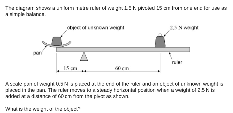
A student recently asked for help with this AQA A-level Physics multiple choice question:

AQA A-level Physics question from 2019 Paper 2

This question is, of course, about Lenz’s Law of Electromagnetic Induction. The law can be stated easily enough: ‘An induced current will flow in a direction so that it opposes the change producing it.’ However, it can be hard for students to learn how to apply it.

What follows is my suggested explanatory sequence.

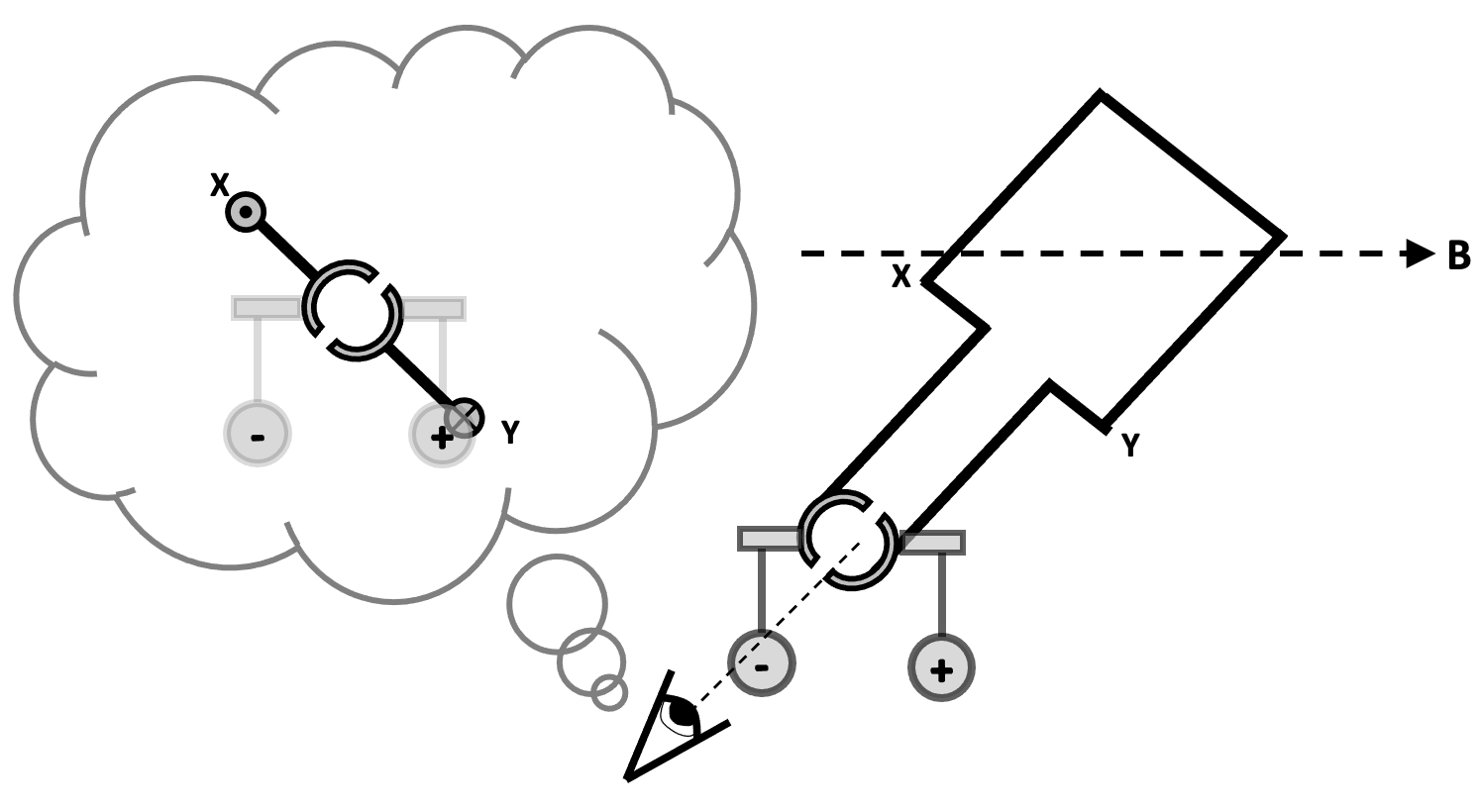
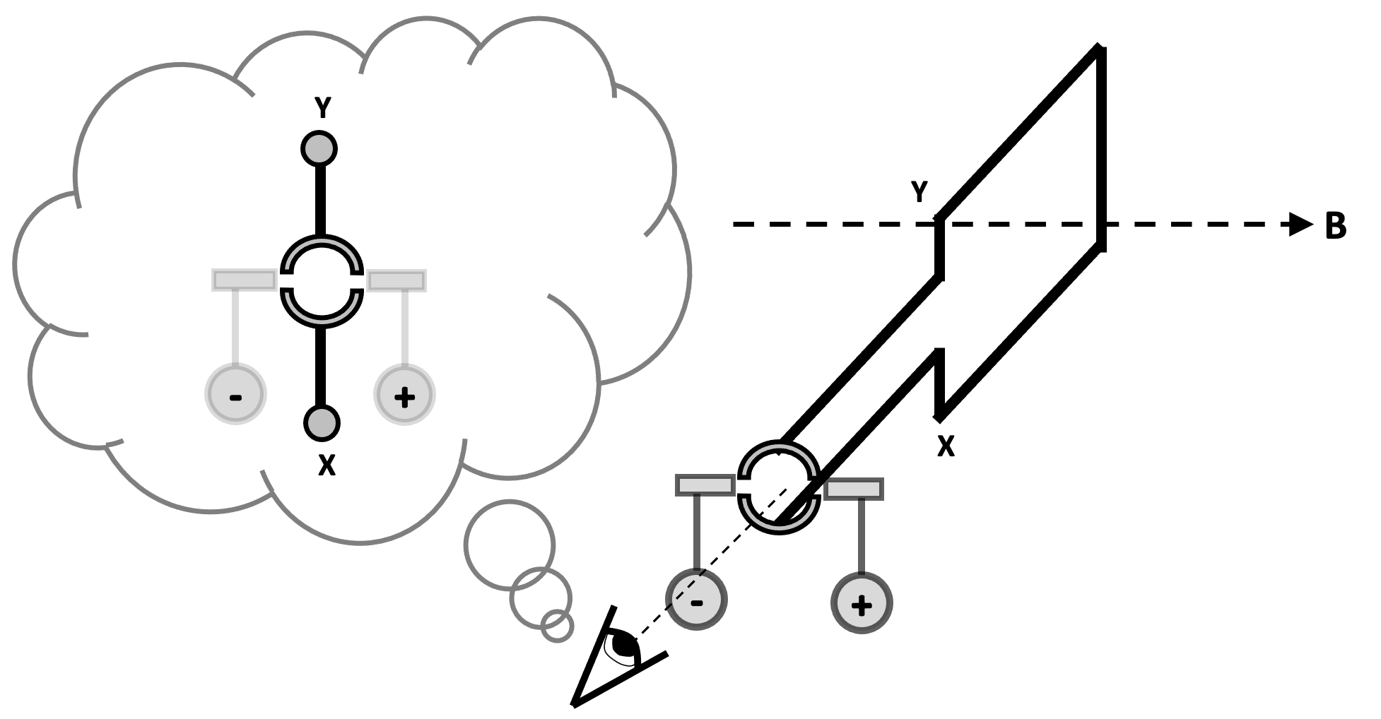
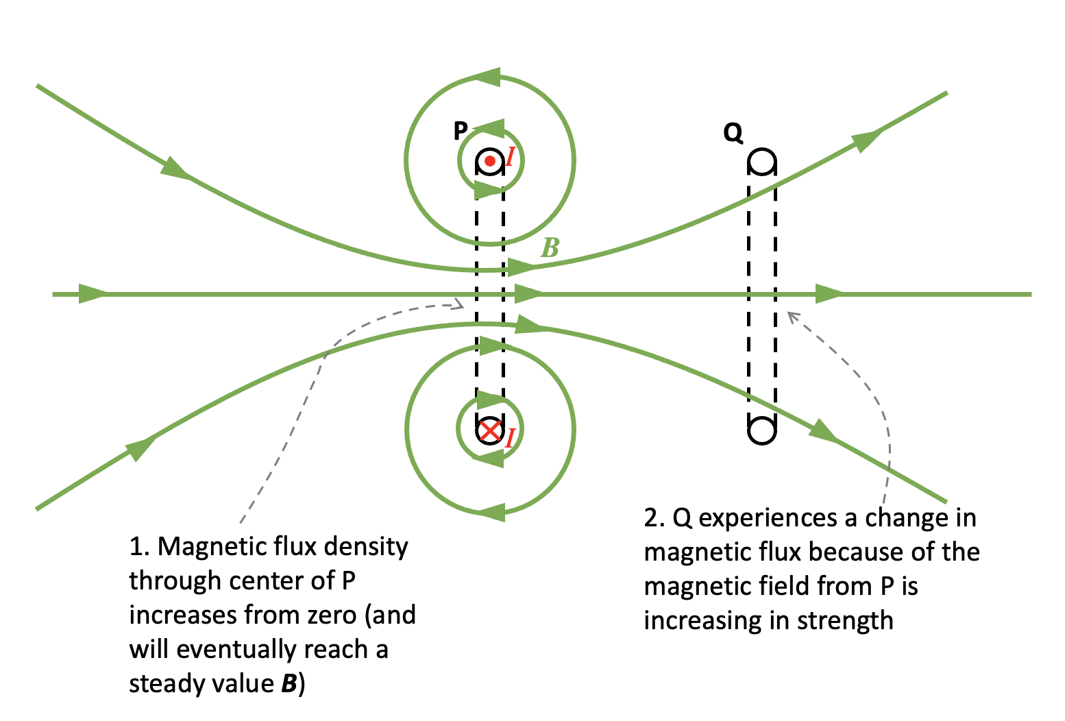
Step 1: simplify the diagram using the ‘dot and cross’ convention

When the switch is closed, a current I begins to flow in coil P. We can assume that I starts at zero and increases to a maximum value in a very small but not negligible period of time.

Simplified 2D representation of the top diagram. The current directions I are arbitrary based on my ‘best guess’ interpretation of the 3D diagram and could be reversed if desired.

Step 2: consider the magnetic field produced by P

You can read more about a simple method of deducing the direction of the magnetic field produced by a coil or a solenoid here.

Step 3: apply Faraday’s Law to coil Q

Since Q is experiencing a change in magnetic flux, then an induced current will flow through it.

Step 4: apply Lenz’s Law to coil Q

The current in coil Q must flow in such a direction so that it opposes the change producing it.

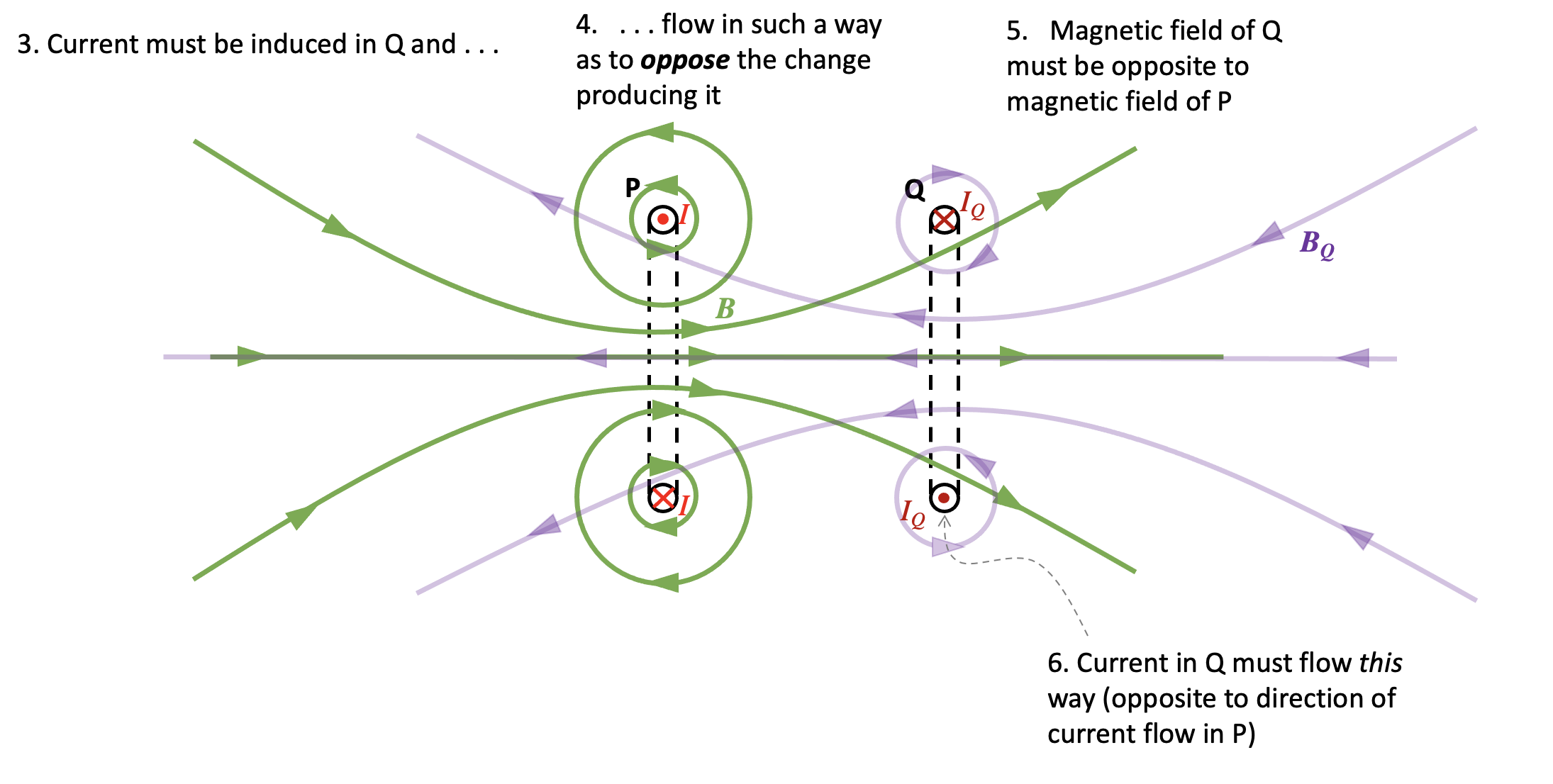
Since P is producing an increasing magnetic flux through Q, then the current in Q must flow in such a way so that it tries to prevent the increase in magnetic flux which is inducing it. The direction of the magnetic field BQ produced by Q must therefore be opposite to the direction of the magnetic field produced by P.

Step 5: consider the polarity of the magnetic fields of P and Q

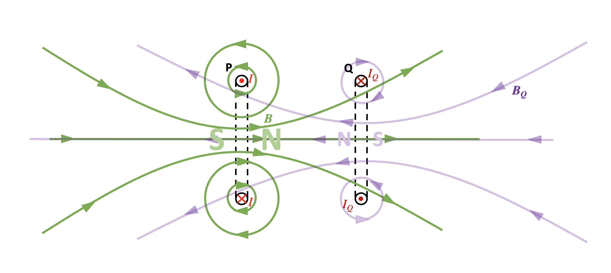
We can see the magnetic field lines of coil P produce a north magnetic field on its right hand side. The magnetic field of Q will produce a north magnetic field on its left hand side. Coil P will therefore push coil Q to the right.

It follows that we can eliminate options A and C from the question.

Step 6: What happens when the magnetic field of P reaches its steady value?

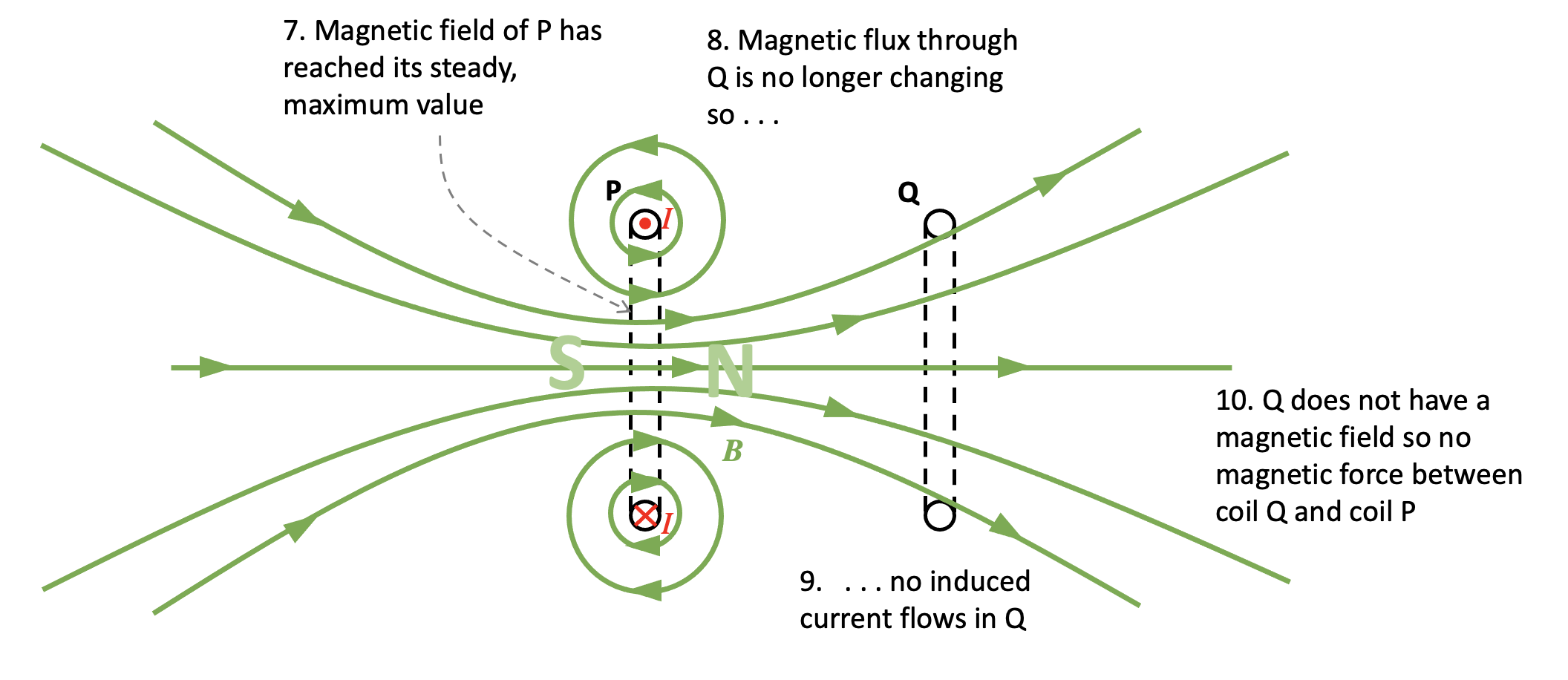
Because the magnetic field produced by coil P has how reached its steady maximum value, this means that the magnetic flux through coil Q also has a constant, unchanging value. Since there is no change in magnetic flux, then this means that no emf is induced across the coil so no induced current flows. Since Q does not have a magnetic field it follows that there is no magnetic interaction between them.

The answer to the question must therefore be D.

Step 7: check student understanding

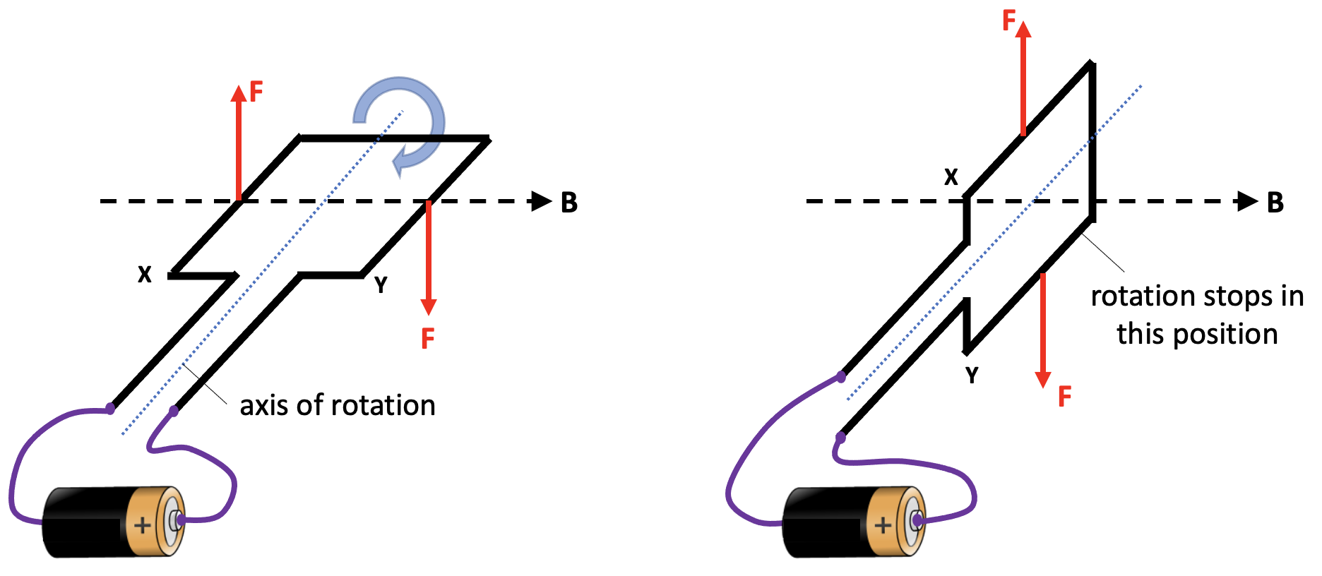
For the alternative question, the correct answer of C can be explained by going through a process similar to the one outlined above.

  • When the switch is opened, the magnetic flux through Y begins to decrease.
  • A changing magnetic flux through Y induces current flow.
  • Lenz’s Law predicts that the direction of this current is such that it opposes the change producing it.
  • The current through Y will therefore be in the same direction as the current through X to produce a magnetic field in the same direction.
  • The coils will attract each other.
  • Eventually, the magnetic flux produced by coil X drops to a constant value of zero.
  • Since there is no change in magnetic flux through Y, there is no induced current flow through Y and hence no magnetic field.
  • There is no magnetic interaction between X and Y and therefore the force on Y is zero.

Conclusion

I hope teachers find this detailed analysis of a Lenz’s Law question useful! As in much of A-level Physics, the devil is not in the detail but rather in the application of the detail. Students who encounter more examples will have a more secure understanding.

Reference

Griffiths, David (2013). Introduction to Electrodynamics. p. 315.

Dual coding change of momentum

Rosencrantz (an anguished cry): CONSISTENCY IS ALL I ASK!

Tom Stoppard, Rosencrantz and Guildenstern Are Dead (1966)

I think that dual coding techniques can be extremely helpful in helping students understand the concept of change of momentum.

To engage our students’ physical intuitions, let’s consider a question like: Which would hurt more — being hit by a sandbag or being hit by a rubber ball?

Let’s assume that the sandbag and rubber ball have the same mass m and are travelling at the same initial velocity u. We choose ‘u‘ because it’s the initial velocity and we take ‘v‘ as the final velocity: a very subtle piece of dual coding that can reap rewards if applied consistently — pace Rosencrantz(!) — over a range of disparate examples.

To analyse this problem, let’s use the momentum version of Newton’s Second Law of Motion.

We will use the change = final – initial convention (‘Consistency is all I ask!’)). The initial momentum is pi and the final momentum is pf.

Now let’s work out the change in momentum in each case. We will assume that each item is dropped so that it impacts vertically on a horizontal surface. The velocity just before it hits is u so its initial momentum pi is given by pi = mu; its final velocity is v so its final momentum pf is given by pf = mv. The sandbag does not rebound, so its final velocity v is zero.

The rubber ball rebounds from the surface with a velocity v (we have shown that v < u so we are not assuming a perfectly elastic collision).

We will use the down-is-positive convention so that u is positive and the downward momentum pi are positive in both cases. However, the velocity v of the ball is negative so the momentum pf = mv is negative (upwards).

To add vectors, we simply put them ‘nose to tail’. However, in this case, we need to subtract the vectors, not add them. To do this, we use the operation pf + (-pi,). In other words, we put the vector pf nose to tail with minus pi, or with a vector pointing in the opposite direction to the original vector pi. These are shown in the table.

We can see that the change in momentum Δp is larger in the case of the rubber ball.

Applying Newton Second Law that force = change in momentum / change in time then (assuming the time of each interaction is the same) then we can conclude that the (upward) force exerted by the surface on the ball is larger than the force exerted by the surface on the sandbag.

From Newton’s Third Law (that if an object A exerts a force on object B, then object B exerts an equal and opposite force on object A), we can also conclude that the rubber exerts a larger downward force on the surface. This implies that, if the ball hit (say) your hand, then it would hurt more than the sandbag.

Considering change of momentum problems like this helps students answer questions such as the one shown below:

Exam question on change in momentum (solid black arrow and red arrow added)

We can discard options C and D since the change of momentum shown is in the wrong direction: the vertical component of momentum will remain unchanged.

A and B show changes of momentum of the same magnitude in the horizontal direction. However, if we take the horizontal component of the initial momentum as positive then the change of momentum on the gas particle must be negative; this implies that the correct answer is B.

Note also that diagram B shows the pf + (-pi) operation outlined above, with the arrow showing minus pi shown in red (added to the original exam question).

Introducing vectors (part 2)

This post suggests some strategies for teaching vectors to 14-16 olds. In part 1 we looked at the idea of combining two vectors into one; that is to say, finding the resultant vector. In this part, we’re going to look at the inverse operation: splitting a single vector into two component vectors.

We’re going to use scale drawing rather than trigonometry since (a) this often leads to a more secure understanding; and (b) it is the expected method in the UK curriculum for 14-16 year olds.

What is a component vector?

A component vector is one of at least two vectors that will combine to give one single original vector. The component vectors are chosen so that they are mutually perpendicular. Because of this, they cannot affect each other’s magnitude and direction and so can be dealt with separately and independently; that is to say, we can choose to consider what effect the vertical component will have on its own without having to worry about what effect the horizontal component will have.

Introducing components as ‘the vector less travelled by’

Two roads diverged in a wood, and I—
I took the one less traveled by,
And that has made all the difference.

Robert Frost, 'The Road Less Travelled'

Let’s say we travelled a distance of 13 m from point O to point P on a compass bearing of 067 degrees (bear with me, I’m working with a slightly less familiar Pythagorean 3:4:5 triple here). This could be drawn as a scale diagram as shown below.

Could we analyse the displacement OP in terms of an eastward displacement and a northward displacement?

We can — as shown below.

The dotted line OX is the eastward (horizontal on our diagram) component of the displacement OP. It is drawn as a dotted line because it is (literally) the ‘road less travelled’. We did not walk along that road — and that’s why it is drawn as a dotted line — but we could have done.

But let’s say that we had, and that we had stopped when we reached the point marked X. And then we look around, and strike out northwards and walk the (vertical) ‘road less travelled called XP — and we end up at P.

So walking one road less travelled might, indeed, make ‘all the difference’ — but walking two roads less travelled does not.

To rewrite Robert Frost: We took the two roads less travelled by / And that has made NO difference.

But why should we wish to go the ‘long way around’, even if we still end up at P? Because it would allow us to work out the change in longitude and latitude. By moving from O to P we change our longitude by 12 metres and our latitude by 5 metres. (Don’t believe me? Count the squares on the diagram!)

We have resolved the 13 metre distance into two components: one eastward (horizontal) component of 12 metres and one northward component of 5 metres.

Using resolving a vector into components to solve problems

We can use the scale drawing technique outlined above to resolve (‘split’) the 3000 N vector into a horizontal component and a vertical component.

The full solution is shown in sequence on this PowerPoint.

Gravitational potential: the ‘bottom of a hole’ perspective

The surface of Mars imaged by NASA’s Curiosity rover in 2013

April 20, 2112: The sky is flat, the land is flat, and they meet in a circle at infinity. No star shows but the big one, a little bigger than it shows through most of the [asteroid] Belt, but dimmed to red, like the sky. It’s the bottom of a hole, and I must have been crazy to risk it. […] The stars are gone, and the land around me makes no sense. Now I know why they call planet dwellers ‘flatlanders’. I feel like a gnat on a table. I’m sitting here shaking, afraid to step outside. […] I’M AT THE BOTTOM OF A LOUSY HOLE!

Larry Niven, ‘At The Bottom of a Hole’ (1966)

Redish and Kuo (2015: 586) suggest that tapping into our students’ innate physical intuitions can be a very productive teaching strategy. For example, Redish observed some physics instructors teaching non-physics majors how to interpret a potential energy U against the separation r between particles graph (diagram 8(a) below).

From Redish and Kuo (2015)

The students were finding it difficult to answer the question of whether the particles would attract or repel each other when they had energy E and were at a separation of C. Redish noted that the instructors advised the students to consider the derivative of the curve at C (diagram 8(b) above) and, since it had a positive gradient, to surmise that the force between the particles would therefore be attractive since F=-dU/dr. Redish suggested:

A more effective approach for this population might be to begin with an embodied analogy and implicitly supporting epistemologies valuing physical intuition. Start with treating a potential energy curve as a track or hill and, using the analogy of gravitational potential energy, then place a ball on the hill as shown in Fig. 8c.

Redish and Kuo (2015)

Which way would the ball roll in 8(c) roll? Redish said that the students had no problem deducing that the particles would exert an attractive force on each other at C (and a repulsive force when their energy is E at the smaller value of r) after using this analogy.

Using students’ physical intuitions to help understand gravitational potential

The episode outlined above reminded me of a science fiction story by Larry Niven that I had read many years ago. In ‘At the Bottom of a Hole’, Niven imagined what landing on a planet would feel like to a ‘Belter’; that is to say, to a human being who had spent their entire life navigating between the small worlds of the asteroid Belt: small planetoid-sized worlds whose shallow gravitational fields required only a low-intensity burn for a spaceship to slip free of their influence forever. An extract from the story is quoted as an introduction to this post: in essence, the ‘Belter’ who has lived his life voyaging between the low mass and low gravity worldlets of the asteroid belt finds it emotionally and psychologically disturbing to find himself at the bottom of a deep gravitational hole.

Gravitational Fields are always ‘holes’

Gravitational fields are always holes (unlike electric fields, of course, which can be either ‘holes’ or ‘mountains’; this may well form the basis of a later post).

The mass of the Earth produces a much deeper gravitational hole than the much smaller mass of an asteroid.

As a consequence, a spaceship near the Earth’s surface (A) needs to burn a lot more fuel (i.e. do a lot more work) to completely escape the gravitational influence of the Earth (B) then a spaceship near to the surface of an asteroid. The spaceship closer to the asteroid (C) needs a much smaller burn to completely escape its gravitational influence (D).

To a mature space-faring civilisation, living on the surface of a planet could well be likened (and seem as eccentric) as living at the bottom of a spectacularly deep hole.

Gravitational potential

The gravitational potential of an object of mass M is given by:

where G is the Gravitational Constant and r is the displacement from the centre of mass of the object. The units of V would be joules per kilogram J/kg.

Note that the magnitude of V gets larger as r decreases. This allows us to represent a gravitational field in terms of equipotential lines (dotted on the diagram below) as well as field lines (solid).

Modelling gravitational potential as a three dimensional hole

We can engage our own and our students’ physical intuitions by picturing the equipotential lines as being contour lines indicating the depth of a three dimensional hole.

An object represented as a ball at position A will not tend to roll down into the hole since there is no discernible downhill ‘slope’ at A; in effect, as r tends towards infinity then the object is beyond the effects of M’s gravity. A position outside the gravitational field of a massive object has a gravitational potential of zero.

Let’s think about what happens as r decreases until the object is at B. Here we can intuitively surmise that it will experience a small force tending to make it fall deeper into the hole. How much work will the gravitational field have done moving an object from infinity to this position? The answer is, of course, 0.5 MJ for each kilogram of mass.

How much work will be done by the gravitational field moving the object from B to C? The answer is again an extra 0.5 MJ/kg but note that this happens over a much smaller change in r than before because the gravitational field is becoming more intense. Again, we can intuit that the object will experience a stronger gravitational force at C than at B.

We can go on to argue that a similar pattern of behaviour will also occur at D and E.

But the real value of this representation is, in my opinion, helping students understand how much energy a body needs to escape the influence of a gravitational field.

If we start at B, we would have to do 0.5 MJ/kg of work on it to make it escape. In other words, it needs 0.5 MJ/kg to climb out of the hole.

If we started at C, then we would need 1.0 MJ/kg; and D, 1.5 MJ/kg and so on.

If we were considering a spacecraft operating in the vacuum of space, then transferring 2.0 MJ/kg of kinetic energy would allow ot to completely escape the gravitational influence of M; or, in other words, to reach a value of r such that its gravitational potential is zero.

Near the Earth’s surface where r = 6.38 x 10⁶ m, the gravitational potential can be calculated as follows:

That is to say, a body would need to gain 64.4 MJ of kinetic energy for each kilogram of its mass to completely escape from the influence of the Earth’s gravity.

We can therefore calculate the escape velocity for a body near the Earth surface as follows:

As I mentioned above, I think the real power of this way of tapping into physical intuition for understanding fields comes when we use it to represent electric fields. I will cover that in a later post.

Reference

Redish, E. F., & Kuo, E. (2015). Language of physics, language of math: Disciplinary culture and dynamic epistemologyScience & Education24, 561-590.

The ‘all-in-a-row’ circuit diagram convention for series and parallel circuits

Circuit diagrams can be seen either as pictures or abstractions but it is clear that pupils often find it hard to recognise the circuits in the practical situation of real equipment. Moreover, Caillot found that students retain from their work with diagrams strong images rather than the principles they are intended to establish. The topological arrangement of a diagram or a drawing presents problems for pupils which are easily overlooked. It seems that pupils’ spatial abilities affect their use of circuit diagrams: they sometimes do not regard as identical several circuits, which, though identical, have been rotated so as to have a different spatial arrangement. […] Niedderer found that pupils, when asked whether a circuit diagram would ‘work’ in practice, more often judged symmetrical diagrams to be functioning than non-symmetric ones.

Driver et al. (1994): 124 [Emphases added]

For the reasons outlined by Driver and others above, I think it’s a good idea to vary the way that we present circuit diagrams to students when teaching electric circuits. If students always see circuit diagrams presented so that (say) the cell is at the ‘top’ and ‘facing’ a certain way; or that they are drawn so that they are symmetrical (which is an aesthetic rather that a scientific choice), then they may well incorrectly infer that these and other ‘accidental’ features of our circuit diagrams are the essential aspects that they should pay the most attention to.

One ‘shake it up’ strategy is to redraw a circuit diagram using the ‘all-in-a-row’ convention.

If you arrange the real components in the ‘all-in-a-row’ arrangement, then a standard digital voltmeter has, what is in my opinion a regrettably underused functionality, that will show:

  • ‘positive’ potential differences: that is to say, the energy added to the coulombs as they pass through a cell or the electromotive force; and
  • ‘negative’ potential differences: that is to say, the energy removed from each coulomb as they pass through a resistor; these can be usefully referred to as ‘potential drops’

This can be shown on circuit diagrams as shown below/

In other words, the difference between the potential difference across the cell (energy being transferred into the circuit from the chemical energy store of the cell) is explicitly distinguished from the potential difference across the resistor (energy being transferred from the resistor into the thermal energy store of the surroundings). The all-in-a-row convention neatly sidesteps a common misconception that the potential difference across a cell is equal to the potential difference across a resistor: they are not. While they may be numerically equal, they are different in sign, as a consequence of Kirchoff’s Second Law. As I have suggested before, I think that this misconception is due to the ‘hidden rotation‘ built into standard circuit diagrams.

Potential divider circuits and the all-in-a-row convention

Although I am normally a strong proponent of the ‘parallel first heresy‘, I’ll go with the flow of ‘series circuit first’ in this post.

Diagrams 2 and 3 in the sequence show that the energy supplied to the coulombs (+1.5 V or 1.5 joules per coulomb) by the cell is transferred from the coulombs as they pass through the double resistor combination. Assuming that R1 = R2 then, as diagram 4 shows, 0.75 joules will be transferred out of each coulomb as they pass through R1; as diagram 5 shows, 0.75 joules will be transferred out of each coulomb as they pass through R2.

Parallel circuits and the all-in-a-row convention

I’ve written about using the all-in-a-row convention to help explain current flow in parallel circuits here, so I will focus on understanding potential difference in parallel circuit in this post.

Again, diagrams 2 and 3 in the sequence show that the positive 3.0 V potential difference supplied by the cell is numerically equal (but opposite in sign) to the negative 3.0 V potential drop across the double resistor combination. It is worth bearing in mind that each coulomb passing through the cell gains 3.0 joules of energy from the chemical energy store of the cell. Diagrams 4 and 5 show that each coulomb passing through either R1 or R1 loses its entire 3.0 joules of energy as it passes through that resistor. The all-in-a-row convention is useful, I think, for showing that each coulomb passes through just one resistor as it makes a single journey around the circuit.

Acknowledgements

Circuit simulations from the excellent https://phet.colorado.edu/sims/html/circuit-construction-kit-dc/latest/circuit-construction-kit-dc_en.html

Circuit diagrams drawn using https://www.circuit-diagram.org/editor/

Reference

Driver, R., Squires, A., Rushworth, P., & Wood-Robinson, V. (1994). Making sense of secondary science: Research into children’s ideas. Routledge.

Just a moment . . .

Many years ago, I was taught this compact and intuitive convention to show turning moments. I think it should be more widely known, as it not only is concise and powerful, but also meets the criterion of being an effective form of dual coding which is helpful for both GCSE and A-level Physics students.

Let’s look at an example question.

Let’s start by ‘annotating the hell’ out of the diagram.

We could take moments around any of the marked points A-E on the diagram. However, we’re going to take moments around B as it enables us to ignore the upward reaction force acting on the rule at B. (This force is not shown on the diagram.)

To indicate that we’re going to be considering the sum of the clockwise moments about point B, we use this intuitive notation:

If we consider the sum of anticlockwise moments about point B, we use this:

We lay out our calculations of the total clockwise and anticlockwise moments about B as follows.

We show that we are going to apply the Principle of Moments (the sum of clockwise moments is equal to the sum of anticlockwise moments for an object in equilibrium) like this:

The rest, as they say, is not history but algebra:

I hope you find this ‘momentary’ convention useful(!)

Split ring commutator? More like split ring commuHATER!

Students find learning about electric motors difficult because:

  1. They find it hard to predict the direction of the force produced on a conductor in a magnetic field, either with or without Fleming’s Left Hand Rule.
  2. They find it hard to understand how a split ring commutator works.

In this post, I want to focus on a suggested teaching sequence for the action of a split ring commutator, since I’ve covered the first point in previous posts.

Who needs a ‘split ring commutator’ anyway?

We all do, if we are going to build electric motors that produce a continuous turning motion.

If we naively connected the ends of a coil to power supply, then the coil would make a partial turn and then lock in place, as shown below. When the coil is in the vertical position, then neither of the Fleming’s Left Hand Rule (FLHR) forces will produce a turning moment around the axis of rotation.

When the coil moves into this vertical position, two things would need to happen in order to keep the coil rotating continuously in the same direction.

  • The current to the coil needs to be stopped at this point, because the FLHR forces acting at this moment would tend to hold the coil stationary in a vertical position. If the current was cut at this time, then the momentum of the moving coil would tend to keep it moving past this ‘sticking point’.
  • The direction of the current needs to be reversed at this point so that we get a downward FLHR force acting on side X and an upward FLHR force acting on side Y. This combination of forces would keep the coil rotating clockwise.

This sounds like a tall order, but a little device known as a split ring commutator can help here.

One (split) ring to rotate them all

The word commutator shares the same root as commute and comes from the Latin commutare (‘com-‘ = all and ‘-mutare‘ = change) and essentially means ‘everything changes’. In the 1840s it was adopted as the name for an apparatus that ‘reverses the direction of electrical current from a battery without changing the arrangement of the conductors’.

In the context of this post, commutator refers to a rotary switch that periodically reverses the current between the coil and the external circuit. This rotary switch takes the form of a conductive ring with two gaps: hence split ring.

Tracking the rotation of a coil through a whole rotation

In this picture below, we show the coil connected to a dc power supply via two ‘brushes’ which rest against the split ring commutator (SRC). Current is flowing towards us through side X of the coil and away from us through side Y of the coil (as shown by the dot and cross 2D version of the diagram. This produces an upward FLHR force on side X and a downward FLHR force on side Y which makes the coil rotate clockwise.

Now let’s look at the coil when it has turned 45 degrees. We note that the SRC has also turned by 45 degrees. However, it is still in contact with the brushes that supply the current. The forces on side X and side Y are as noted before so the coil continues to turn clockwise.

Next, we look at the situation when the coil has turned by another 45 degrees. The coil is now in a vertical position. However, we see that the gaps in the SRC are now opposite the brushes. This means that no current is being supplied to the coil at this point, so there are no FLHR forces acting on sides X and side Y. The coil is free to continue rotating clockwise because of momentum.

Let’s now look at the situation when the coil has rotated a further 45 degrees to the orientation shown below. Note that the side of the SRC connected to X is now touching the brush connected to the positive side of the power supply. This means that current is now flowing away from us through side X (whereas previously it was flowing towards us). The current has reversed direction. This creates a downward FLHR force on side X and an upward FLHR force on side Y (since the current in Y has also reversed direction).

And a short time later when the coil has moved a total of180 degrees from its starting point, we can observe:

And later:

And later still:

And then:

And then eventually we get back to:

Summary

In short, a split ring commutator is a rotary switch in a dc electric motor that reverses the current direction through the coil each half turn to keep it rotating continuously.

A powerpoint of the images used is here:

And a worksheet that students can annotate (and draw the 2D versions of the diagrams!) is here:

I hope that this teaching sequence will allow more students to be comfortable with the concept of a split ring commutator — anything that results in a fewer split ring commuHATERS would be a win for me 😉

Speed of sound using Phyphox

You can get encouragingly accurate values for the speed of sound in the school laboratory using a tape measure and two smartphones (or tablets) running the Phyphox app.

Phyphox (pronounced FEE-fox) is an award-winning free app that was developed by physicists at Aachen University who wanted to give users direct access to the many sensors (e.g. accelerometers and magnetometers) which are standard features on many smartphones. In effect, it turns even the humblest smartphone or tablet into a multifunctional measuring instrument comparable to one of Star Trek’s famous ‘tricorders’.

Star Trek Tricorder (not Phyphox)

To measure the speed of sound, we need two smartphones or tablets running Phyphox. We will be using the ‘Acoustic Stopwatch’ which measures the time between two acoustic events.

Phyphox main screen

Step 1: Place two devices a measured distance s apart. Typically about 2 or 3 m should be OK otherwise the sound made by A will not be loud enough to control stopwatch B — this can be established through trial and error and depends on many factors including the background noise level.

Step 2: Person A makes a loud sound (a clap or a single syllable shout like ‘Hey!’ is good).

Step 3: Person B and stopwatch B wait for sound created by A to reach them.
Step 4: The sound reaches stopwatch B and starts it running and B hears the sound.

Step 5: B makes a loud sound in response.

Step 6: The loud sound made by B reaches stopwatch B and makes it stop. Let’s call the time displayed tB. This measures the delay between the sound from A reaching stopwatch B and B reacting to the sound and stopping the clock. It includes the time taken for the initial sound travelling from the device to B, B’s reaction time, and the time taken for the sound made by B to travel to stopwatch B. B does not have to be particularly ‘quick off the mark’ to respond to A’s sound — although the shorter the time then the less likely it is then a background noise will interrupt the experiment.

Step 7: The sound made by B travels toward stopwatch A.

Step 8: The sound made by B reaches stopwatch A and makes it stop. Let’s call the time recorded on stopwatch A tA.

If we break down the events included in tA and tB, we find that tA is always larger than tB:

If we subtract tAtB we find that this is the time it takes sound to travel a distance of 2s.

Step 9: We can therefore use this formula to find the v the speed of sound.

We have found that this method works well giving mean values of about 350 m/s for the speed of sound (which will vary with air temperature). This video models the method.

And so we have a reasonably practicable method of measuring the speed of that doesn’t involve complex equipment that is unfamiliar to most students; or a method that involves finding a large and featureless wall that produces a detectable echo when a loud sound is made from a point several metres in front of it.

I don’t know about you, but as a physics teacher, I feel cheated. If it doesn’t involve a double beam oscilloscope, a signal generator, two microphones and two power amplifiers then I simply don’t want to know about it . . .

The Rite of AshkEnte, quite simply, summons and binds Death.  Students of the occult will be aware that it can be performed with a simple incantation, three small bits of wood and 4cc of mouse blood, but no wizard worth his pointy hat would dream of doing anything so unimpressive; they knew in their hearts that if a spell didn’t involve big yellow candles, lots of rare incense, circles drawn on the floor with eight different colours of chalk and a few cauldrons around the place then it simply wasn’t worth contemplating.

Terry Pratchett, ‘Mort’ (1987)

Deriving centripetal acceleration

When I was an A-level physics student (many, many years ago, when the world was young LOL) I found the derivation of the centripetal acceleration formula really hard to understand. What follows is a method that I have developed over the years that seems to work well. The PowerPoint is included at the end.

Step 1: consider an object moving on a circular path

Let’s consider an object moving in circular path of radius r at a constant angular speed of ω (omega) radians per second.

The object is moving anticlockwise on the diagram and we show it at two instants which are time t seconds apart. This means that the object has moved an angular distance of ωt radians.

Step 2: consider the linear velocities of the object at these times

The linear velocity is the speed in metres per second and acts at a tangent to the circle, making a right angle with the radius of the circle. We have called the first velocity v1 and the second velocity at the later time v2.

Since the object is moving at a constant angular speed ω and is a fixed radius r from the centre of the circle, the magnitudes of both velocities will be constant and will be given by v = ωr.

Although the magnitude of the linear velocity has not changed, its direction most certainly has. Since acceleration is defined as the change in velocity divided by time, this means that the object has undergone acceleration since velocity is a vector quantity and a change in direction counts as a change, even without a change in magnitude.

Step 3a: Draw a vector diagram of the velocities

We have simply extracted v1 and v2 from the original diagram and placed them nose-to-tail. We have kept their magnitude and direction unchanged during this process.

Step 3b: close the vector diagram to find the resultant

The dark blue arrow is the result of adding v1 and v2. It is not a useful operation in this case because we are interested in the change in velocity not the sum of the velocities, so we will stop there and go back to the drawing board.

Step 3c switch the direction of velocity v1

Since we are interested in the change in velocity, let’s flip the direction of v1 so that it going in the opposite direction. Since it is opposite to v1, we can now call this -v1.

It is preferable to flip v1 rather than v2 since for a change in velocity we typically subtract the initial velocity from the final velocity; that is to say, change in velocity = v2 – v1.

Step 3d: Put the vectors v2 and (-v1) nose-to-tail

Step 3e: close the vector diagram to find the result of adding v2 and (-v1)

The purple arrow shows the result of adding v2 + (-v1); in other words, the purple arrow shows the change in velocity between v1 and v2 due to the change in direction (notwithstanding the fact that the magnitude of both velocities is unchanged).

It is also worth mentioning that that the direction of the purple (v2v1) arrow is in the opposite direction to the radius of the circle: in other words, the change in velocity is directed towards the centre of the circle.

Step 4: Find the angle between v2 and (-v1)

The angle between v2 and (-v1) will be ωt radians.

Step 5: Use the small angle approximation to represent v2-v1 as the arc of a circle

If we assume that ωt is a small angle, then the line representing v2-v1 can be replaced by the arc c of a circle of radius v (where v is the magnitude of the vectors v1 and v2 and v=ωr).

We can then use the familiar relationship that the angle θ (in radians) subtended at the centre of a circle θ = arc length / radius. This lets express the arc length c in terms of ω, t and r.

And finally, we can use the acceleration = change in velocity / time relationship to derive the formula for centripetal acceleration we a = ω2r.


Well, that’s how I would do it. If you would like to use this method or adapt it for your students, then the PowerPoint is attached.

Please Like or leave a comment if you find this useful 🙂

We all adore Caloric

We all adore a Kia-Ora

Advertising slogan for ‘Kia-Ora’ orange drink (c. 1985)

Energy is harder to define than you would think. Nobel laureate Richard Feynman defined ‘energy’ as

a numerical quantity which does not change when something happens. It is not a description of a mechanism, or anything concrete; it is just a strange fact that we can calculate some number and when we finish watching nature go through her tricks and calculate the number again, it is the same. […] It is important to realize that in physics today, we have no knowledge of what energy is. […] It is an abstract thing in that it does not tell us the mechanism or the reasons for the various formulas.

Feynman Lectures on Physics, Vol 1, Lecture 4 Conservation of Energy (1963)

Current secondary school science teaching approaches to energy often picture energy as a ‘quasi-material substance’.

By ‘quasi-material substance’ we mean that ‘energy is like a material substance in how it behaves’ (Fairhurst 2021) and that some of its behaviours can be modelled as, say, an orange liquid (see IoP 2016).

The eight energy stores as suggested by the IoP

And yet, sometimes these well-meaning (and, in my opinion, effective) approaches can draw some dismissive comments from some physicists.

The Simpsons Comic Book Guy character saying "Picturing energy as a quasi-material substance? That teaching approach smacks of the oh-so-discredited 'Caloric' theory of energy to me . . ."
The Simpsons’ Comic Book Guy weighs in the ‘Teaching Energy’ debate

What was the ‘Caloric Theory of Energy’?

To begin with, there was never a ‘Caloric Theory of Energy’ since the concept of energy had not been developed yet; but the Caloric Theory of Heat was an important step along the way.

Caloric was an invisible, weightless and self-repelling fluid that moved from hot objects to cold objects. Antoine Lavoisier (1743-1794) supposed that the total amount of caloric in the universe was constant: in other words, caloric was thought to be a conserved quantity.

Caloric was thought to be a form of ‘subtle matter’ that obeyed physical laws and yet was so attenuated that it was difficult to detect. This seems bizarre to our modern sensibilities and yet Caloric Theory did score some notable successes.

  • Caloric explained how the volume of air changed with temperature. Cold air would absorb caloric and thus expand.
  • The Carnot cycle which describes the maximum efficiency of a heat engine (i.e. a mechanical engine powered by heat) was developed by Sadi Carnot (1796-1832) on the basis of the Caloric Theory

Why Caloric Theory was replaced

It began with Count Rumford in 1798. He published some observations on the manufacturing process of cannons. Cannon barrels had to be drilled or bored out of solid cylinders of metal and this process generated huge quantities of heat. Rumford noted that cannons that had been previously bored produced as much heat as cannons that were being freshly bored for the first time. Caloric Theory suggested that this should not be the case as the older cannons would have lost a great deal of caloric from being previously drilled.

The fact that friction could seemingly generate limitless quantities of caloric strongly suggested that it was not a conserved quantity.

We now understand from the work James Prescott Joule (1818-1889) and Rudolf Clausius (1822-1888) that Caloric Theory had only a part of the big picture: it is energy that is the conserved quantity, not caloric or heat.

As Feynman puts it:

At the time when Carnot lived, the first law of thermodynamics, the conservation of energy, was not known. Carnot’s arguments [using the Caloric Theory] were so carefully drawn, however, that they are valid even though the first law was not known in his time!

Feynman Lectures on Physics, Vol 1, Lecture 44 The Laws of Thermodynamics

In other words, the Caloric Theory is not automatically wrong in all respects — provided, that is, it is combined with the principle of conservation of energy, so that energy in general is conserved, and not just the energy associated with heat.

We now know, of course, that heat is not a form of attenuated ‘subtle matter’ but rather the detectable, cumulative result of the motion of quadrillions of microscopic particles. However, this is a complex picture for novice learners to absorb.

Caloric Theory as a bridging analogy

David Hammer (2000) argues persuasively that certain common student cognitive resources can serve as anchoring conceptions because they align well with physicists’ understanding of a particular topic. An anchoring conception helps to activate useful cognitive resources and a bridging analogy serves as a conduit to help students apply these resources in what is, initially, an unfamiliar situation.

The anchoring conception in this case is students’ understanding of the behaviour of liquids. The useful cognitive resources that are activated when this is brought into play include:

  • the idea of spontaneous flow e.g. water flows downhill;
  • the idea of measurement e.g. we can measure the volume of liquid in a container; and
  • the idea of conservation of volume e.g. if we pour water from a jug into an empty cup then the total volume remains constant.

The bridging analogy which serves as a channel for students to apply these cognitive resources in the context of understanding energy transfers is the idea of ‘energy as a quasi-material substance’ (which can be considered as an iteration of the ‘adapted’ Caloric Theory which includes the conservation of energy).

The bridging analogy helps students understand that:

  • energy can flow spontaneously e.g. from hot to cold;
  • energy can be measured and quantified e.g. we can measure how much energy has been transferred into a thermal energy store; and
  • energy does not appear or disappear: the total amount of energy in a closed system is constant.

Of course, a bridging analogy is not the last word but only the first step along the journey to a more complete understanding of the physics involved in energy transfers. However, I believe the ‘energy as a quasi-material substance’ analogy is very helpful in giving students a ‘sense of mechanism’ in their first encounters with this topic.

Teachers are, of course, free not to use this or other bridging analogies, but I hope that this post has persuaded even my more reluctant colleagues that they need a more substantive argument than a knee jerk ‘energy-as-substance = Caloric Theory = BAD’.


References

Fairhurst P. (2021), Best Evidence in Science Teaching: Teaching Energy. https://www.stem.org.uk/sites/default/files/pages/downloads/BEST_Article_Teaching%20energy.pdfhttps://www.stem.org.uk/sites/default/files/pages/downloads/BEST_Article_Teaching%20energy.pdf [Accessed April 2022]

Hammer, D. (2000). Student resources for learning introductory physicsAmerican Journal of Physics68(S1), S52-S59.

Institute of Physics (2016), Physics Narrative: Shifting Energy Between Stores. Available from https://spark.iop.org/collections/shifting-energy-between-stores-physics-narrative [Accessed April 2022]