In this post, we are going to look at series circuits using the Coulomb Train Model.
The Coulomb Train Model (CTM) is a helpful model for both explaining and predicting the behaviour of real electric circuits which I think is useful for KS3 and KS4 students.
Without further ado, here is a a summary.

A circuit with one resistor
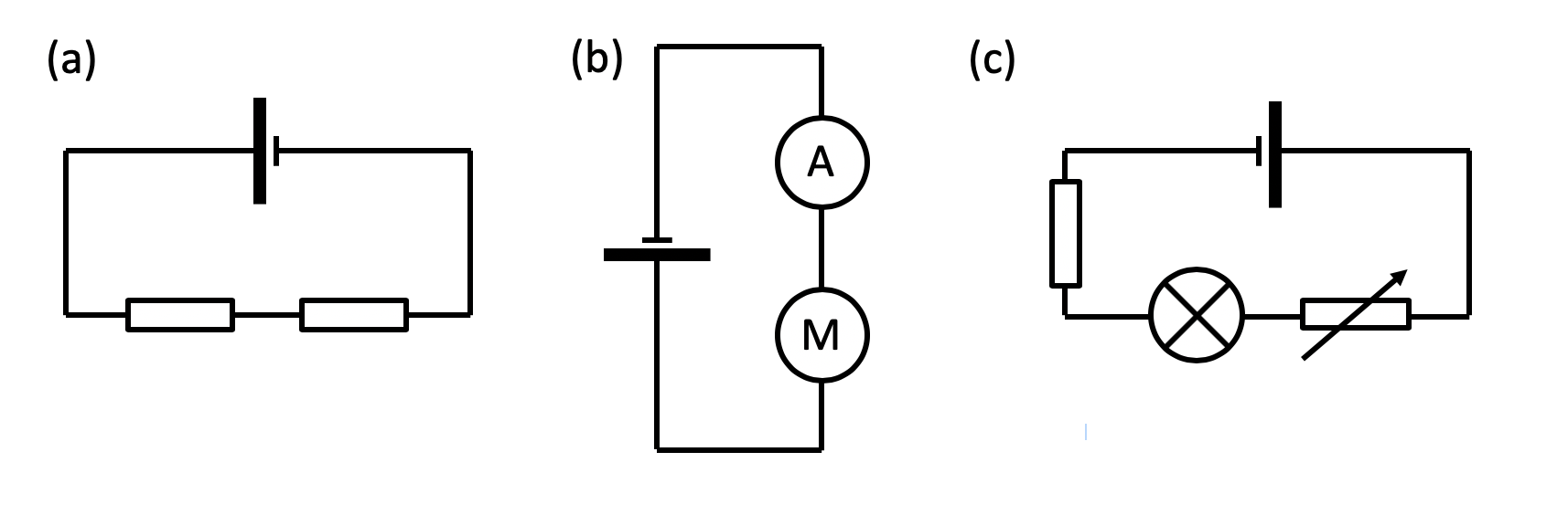
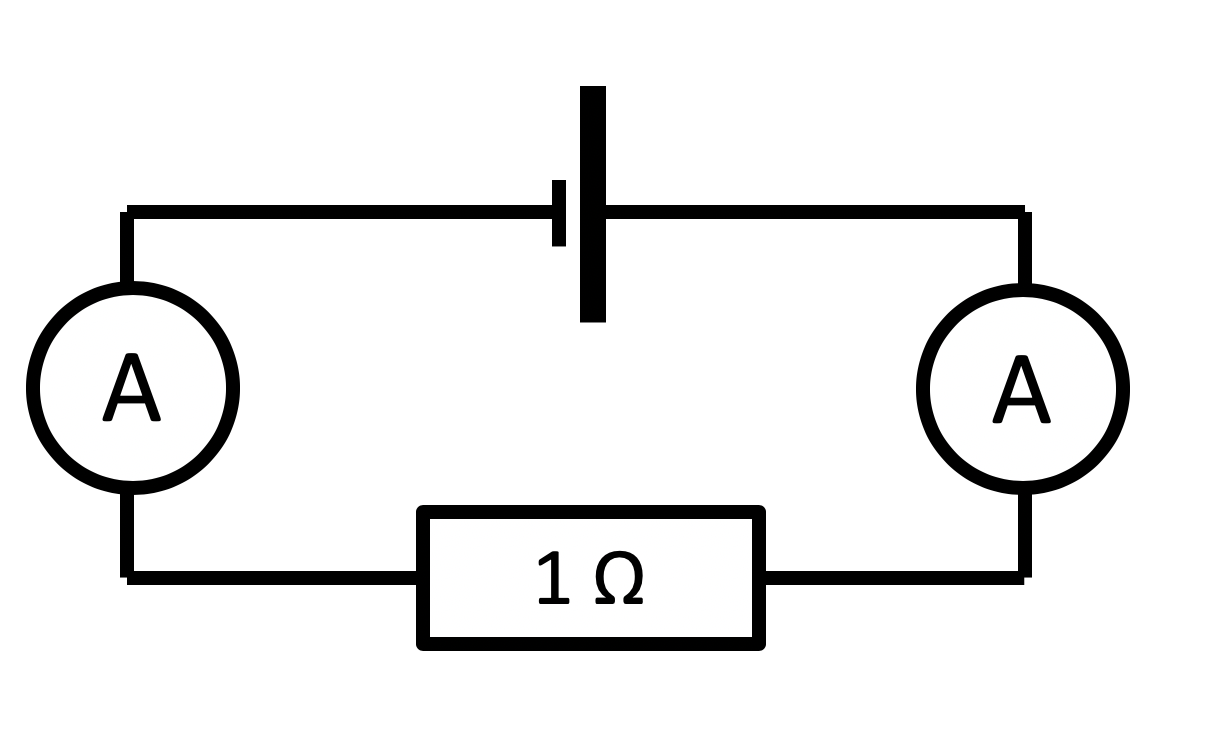
Let’s look at a very simple circuit to begin with:
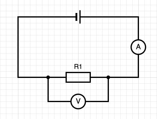
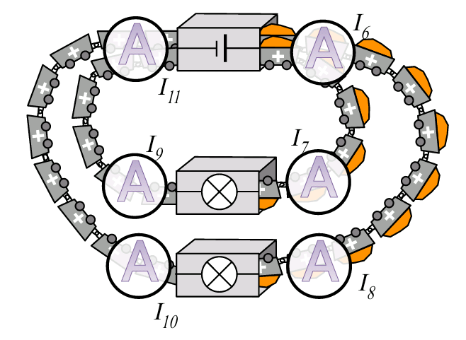
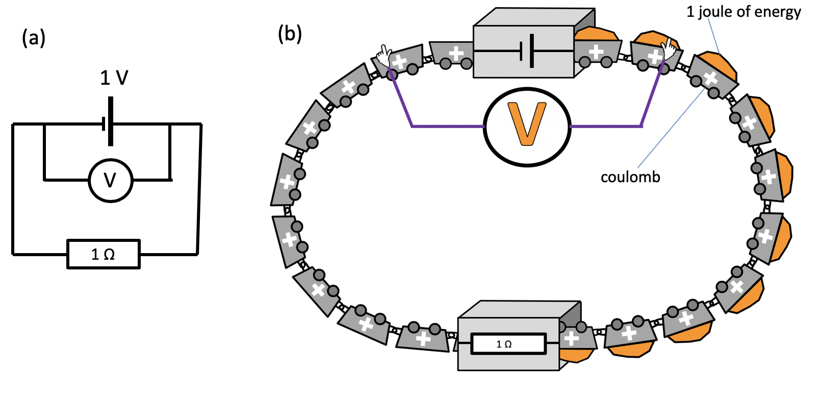
This can be represented on the CTM like this:

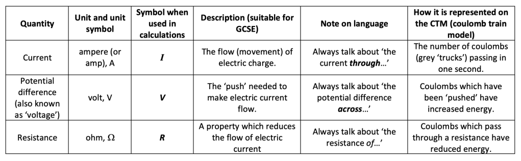
The ammeter counts 5 coulombs passing every 10 seconds, so the current I = charge flow Q / time t = 5 coulombs / 10 seconds = 0.5 amperes.
We assume that the cell has a potential difference of 1.5 V so there is a potential difference of 1.5 V across the resistor R1 (that is to say, each coulomb loses 1.5 J of energy as it passes through R1).
The resistor R1 = potential difference V / current I = 1.5 / 0.5 = 3.0 ohms.
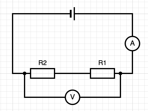
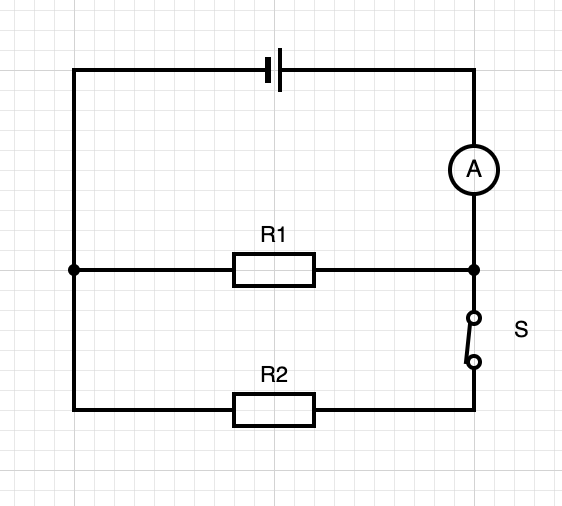
A circuit with two resistors in series
Now let’s add a second identical resistor R2 into the circuit.
This can be shown using the CTM like this:
Notice that the current in this example is smaller than in the first circuit; that is to say, fewer coulombs go through the ammeter in the same time. This is because we have added a second resistor and remember that resistance is a property that reduces the current. (Try and avoid talking about a high resistance ‘slowing down’ the current because in many instances such as two conductors in parallel a high current can be modelled with no change in the speed of the coulombs.)
Notice also that the voltmeter is making identical measurements on both the circuit diagram and the CTM animation. It is measuring the total energy change of the coulombs as they pass through both R1 and R2.
The current I = charge flow Q / time t = 5 coulombs / 20 seconds = 0.25 amps. This is half the value of the current in the first circuit.
We have an identical cell of potential difference 1.5 V the voltmeter would measure 1.5 V. We can calculate the total resistance using R = V / I = 1.5 / 0.25 = 6.0 ohms.
This is to be expected since the total resistance R = R1 + R2 and R1 = 3.0 ohms and R2 = 3.0 ohms.
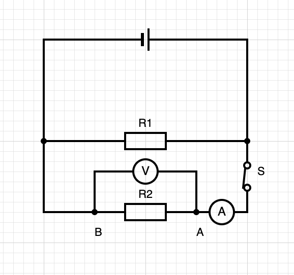
Looking at the resistors individually
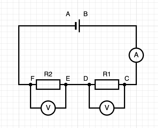
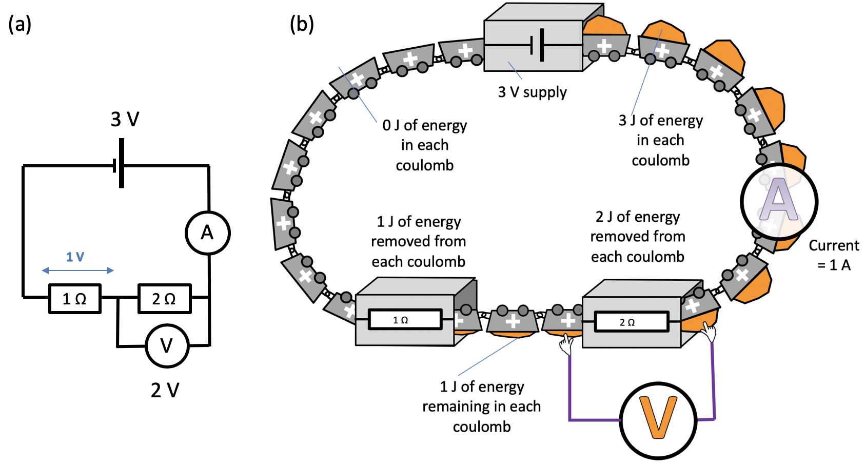
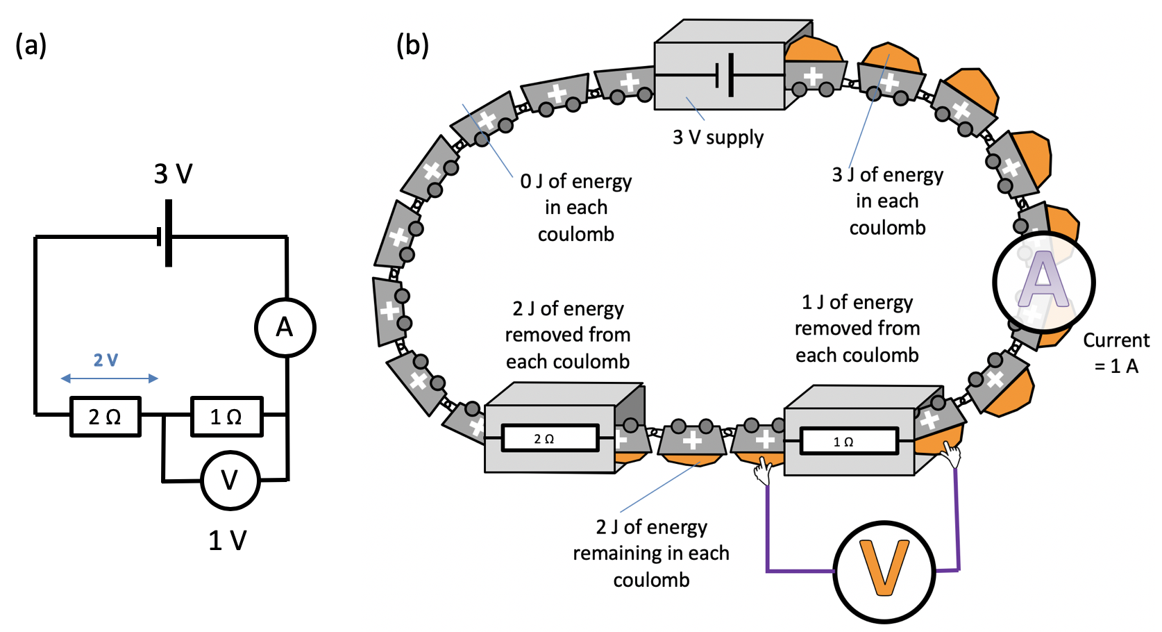
The above circuit can be represented using the CTM as follows:
Between A and B, the coulombs are each gaining 1.5 joules since the cell has a potential difference of 1.5 V. (Remember that V = E energy transferred (in joules) / Q charge flow (in coulombs.)
Between B and C the coulombs lose no energy; that is to say, we are assuming that the connecting wires have negligible resistance.
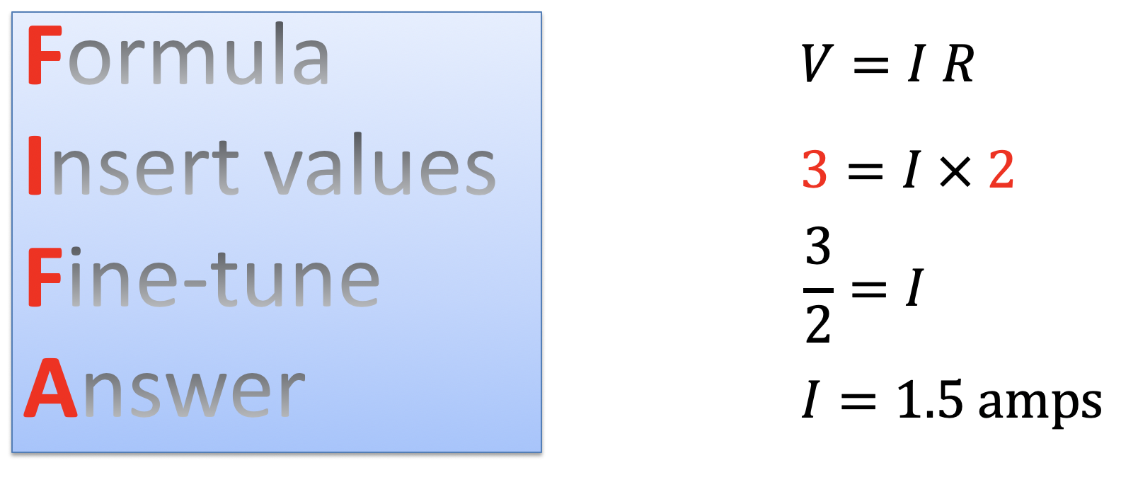
Between C and D the coulombs lose some energy. We can use the familar V = I x R to calculate how much energy is lost from each coulomb, since we know that R1 is 3.0 ohms and I is 0.25 amperes (see previous section).
V = I x R = 0.25 x 3.0 = 0.75 volts.
That is to say, 0.75 joules are removed from each coulomb as they pass through R1 which means that (since 1.5 joules were added to each coulomb by the cell) that 0.75 joules are left in each coulomb.
The coulombs do not lose any energy travelling between D and E because, again, we are assuming negligible resistance in the connecting wire.
0.75 joules is removed from each coulomb between E and F making the potential difference across R2 to be 0.75 volts.
Thus we find that the familiar V = V1 + V2 is a direct consequence of the Principle of Conservation of Energy.
FAQ: ‘How do the coulombs know to drop off only half their energy in R1?’
Simple answer: they don’t.
This may be a valid objection for some donation models of electric circuits (such as the pizza delivery van model) but it doesn’t apply to the CTM because it is a continuous chain model (with the caveat that the CTM applies only to ‘steady state’ circuits where the current is constant).
Let’s look at a numerical argument to support this:
- The magnitude of the current is controlled by only two factors: the potential difference of the cell and the total resistance of the circuit.
- In other words, if we increased the value of R1 to (say) 4 ohms and reduced the value of R2 to 2 ohms so that the total resistance was still 6 ohms, the current would still be 0.25 amps.
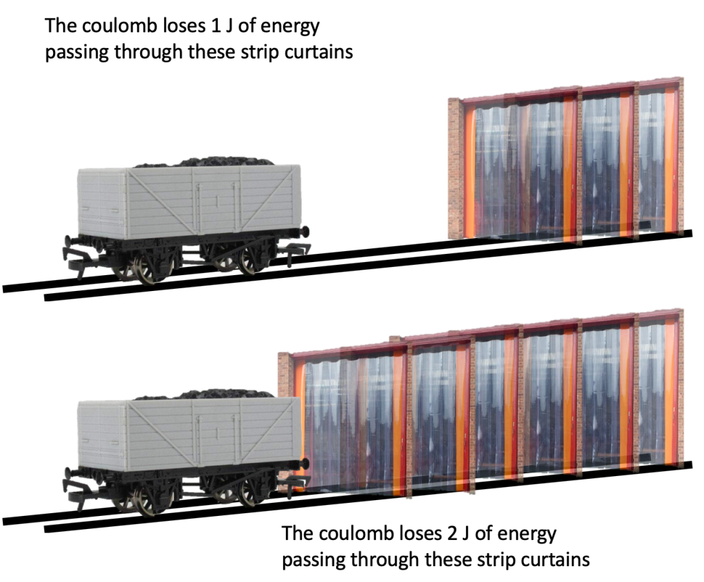
- However, in this case the energy dissipated by each coulomb passing through R1 would V = I x R = 0.25 x 4 = 1 volt (or 1 joule per coulomb) and similarly the potential difference across R2 would now be 0.5 volts.
- The coulombs do not ‘know’ to drop off 1 joule at R1 and 0.5 joules at R2: rather, it is a purely mechanical interaction between the moving coulombs and each resistor.
- R1 has a bigger proportion of the total resistance of the circuit than R2 so it seems self-evident (at least to me) that the coulombs will lose a larger proportion of their total energy passing through R1.
- A similar analysis would apply if we made R2 = 4 ohms and R1 = 2 ohms: the coulombs would now lose 0.5 joules passing through R1 and 1 joule passing through R2.
Thus, we see that the current in a series circuit is affected by the ‘global’ or ‘whole circuit’ properties such as the potential difference of the cell and the total resistance of the circuit. The CTM models this property of real circuits by being a continuous chain of mechanically-linked ‘trucks’ so that a change in any one part of the circuit affects the movement of all the coulombs.
However, the proportion of the energy lost by a coulomb travelling through one part of the circuit is affected — not by ‘magic’ or a weird form of ‘coulomb telepathy’ — but only by the ‘local’ properties of that section of the circuit i.e. the electrical resistance of that section.
(PS You can read more about the CTM and potential divider circuits here.)
Afterword
You may be relieved to hear that this is the last post in my series on ‘The CTM revisited’. My thanks to the readers who have stayed with me through the series (!)
I will close by saying that I have appreciated both the expressions of enthusiasm about CTM and the thoughtful criticisms of it.


 Because the two resistors are identical, the 3 V supply is shared equally across both resistors. That is to say, there is a potential difference of 1.5 V across each resistor. But let’s check this by applying V = IR (eq. 18). The total potential difference is 3 V and the total resistance is 1 ohm + 1 ohm = 2 ohms.