Many years ago, I was taught this compact and intuitive convention to show turning moments. I think it should be more widely known, as it not only is concise and powerful, but also meets the criterion of being an effective form of dual coding which is helpful for both GCSE and A-level Physics students.
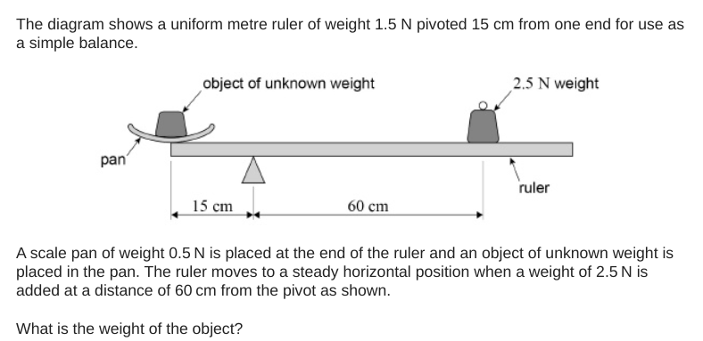
Let’s look at an example question.
Let’s start by ‘annotating the hell’ out of the diagram.
We could take moments around any of the marked points A-E on the diagram. However, we’re going to take moments around B as it enables us to ignore the upward reaction force acting on the rule at B. (This force is not shown on the diagram.)
To indicate that we’re going to be considering the sum of the clockwise moments about point B, we use this intuitive notation:
If we consider the sum of anticlockwise moments about point B, we use this:
We lay out our calculations of the total clockwise and anticlockwise moments about B as follows.
We show that we are going to apply the Principle of Moments (the sum of clockwise moments is equal to the sum of anticlockwise moments for an object in equilibrium) like this:
The rest, as they say, is not history but algebra:
I hope you find this ‘momentary’ convention useful(!)
When I was an A-level physics student (many, many years ago, when the world was young LOL) I found the derivation of the centripetal acceleration formula really hard to understand. What follows is a method that I have developed over the years that seems to work well. The PowerPoint is included at the end.
Step 1: consider an object moving on a circular path
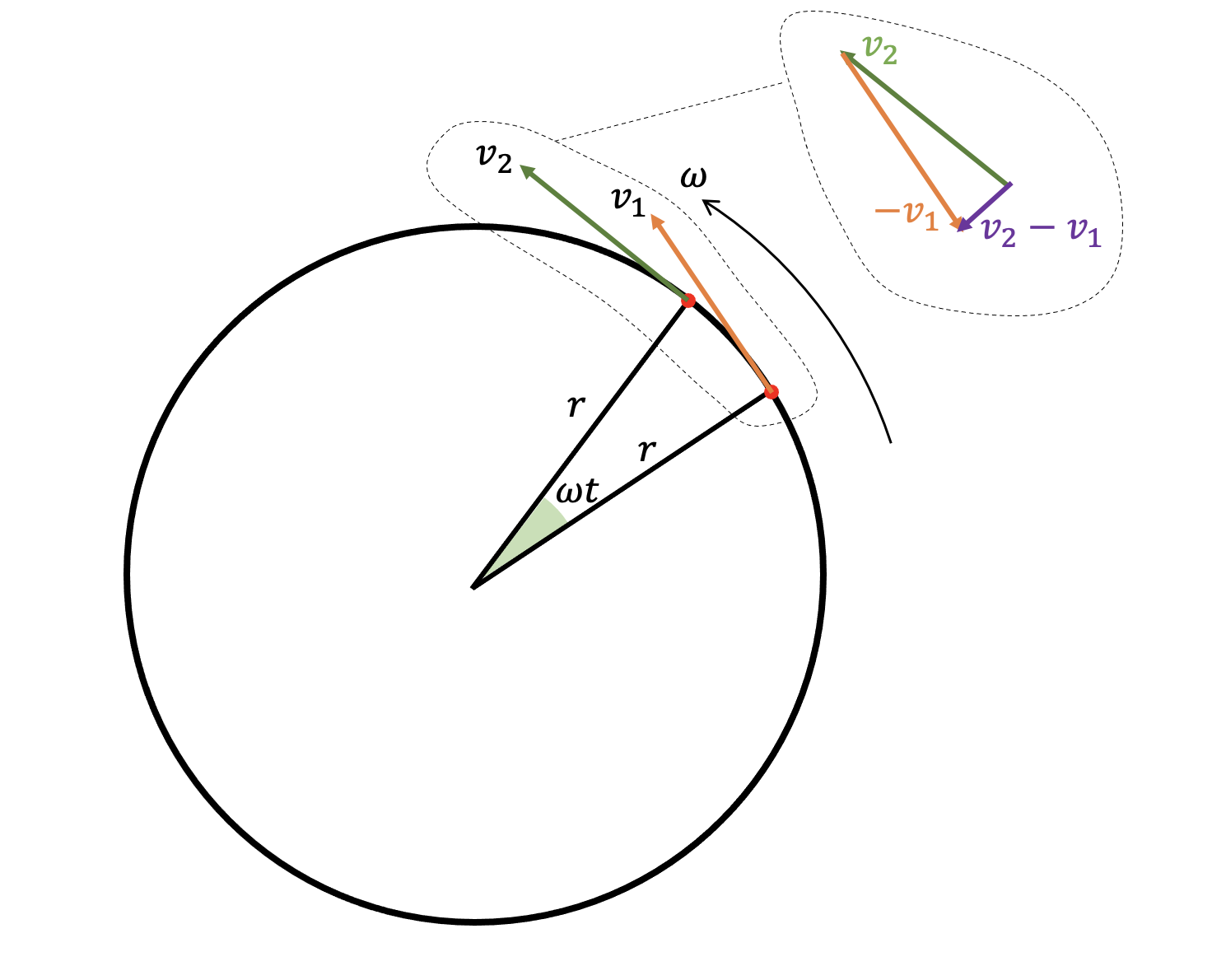
Let’s consider an object moving in circular path of radius r at a constant angular speed of ω (omega) radians per second.
The object is moving anticlockwise on the diagram and we show it at two instants which are time t seconds apart. This means that the object has moved an angular distance of ωt radians.
Step 2: consider the linear velocities of the object at these times
The linear velocity is the speed in metres per second and acts at a tangent to the circle, making a right angle with the radius of the circle. We have called the first velocity v1 and the second velocity at the later time v2.
Since the object is moving at a constant angular speed ω and is a fixed radius r from the centre of the circle, the magnitudes of both velocities will be constant and will be given by v = ωr.
Although the magnitude of the linear velocity has not changed, its direction most certainly has. Since acceleration is defined as the change in velocity divided by time, this means that the object has undergone acceleration since velocity is a vector quantity and a change in direction counts as a change, even without a change in magnitude.
Step 3a: Draw a vector diagram of the velocities
We have simply extracted v1 and v2 from the original diagram and placed them nose-to-tail. We have kept their magnitude and direction unchanged during this process.
Step 3b: close the vector diagram to find the resultant
The dark blue arrow is the result of adding v1 and v2. It is not a useful operation in this case because we are interested in the change in velocity not the sum of the velocities, so we will stop there and go back to the drawing board.
Step 3c switch the direction of velocity v1
Since we are interested in the change in velocity, let’s flip the direction of v1 so that it going in the opposite direction. Since it is opposite to v1, we can now call this -v1.
It is preferable to flip v1 rather than v2 since for a change in velocity we typically subtract the initial velocity from the final velocity; that is to say, change in velocity = v2 – v1.
Step 3d: Put the vectors v2 and (-v1) nose-to-tail
Step 3e: close the vector diagram to find the result of adding v2 and (-v1)
The purple arrow shows the result of adding v2 + (-v1); in other words, the purple arrow shows the change in velocity between v1 and v2 due to the change in direction (notwithstanding the fact that the magnitude of both velocities is unchanged).
It is also worth mentioning that that the direction of the purple (v2 –v1) arrow is in the opposite direction to the radius of the circle: in other words, the change in velocity is directed towards the centre of the circle.
Step 4: Find the angle between v2 and (-v1)
The angle between v2 and (-v1) will be ωt radians.
Step 5: Use the small angle approximation to represent v2-v1 as the arc of a circle
If we assume that ωt is a small angle, then the line representing v2-v1 can be replaced by the arc c of a circle of radius v (where v is the magnitude of the vectors v1 and v2 and v=ωr).
We can then use the familiar relationship that the angle θ (in radians) subtended at the centre of a circle θ = arc length / radius. This lets express the arc length c in terms of ω, t and r.
And finally, we can use the acceleration = change in velocity / time relationship to derive the formula for centripetal acceleration we a = ω2r.
Well, that’s how I would do it. If you would like to use this method or adapt it for your students, then the PowerPoint is attached.
Please Like or leave a comment if you find this useful 🙂
A solenoid is an electromagnet made of a wire in the form of a spiral whose length is larger than its diameter.
A solenoid
The word solenoid literally means ‘pipe-thing‘ since it comes from the Greek word ‘solen‘ for ‘pipe’ and ‘-oid‘ for ‘thing’.
An alternate universe version of the Troggs’ famous 1966 hit record
And they are such an all-embracingly useful bit of kit that one might imagine an alternate universe where The Troggs might have sang:
Pipe-thing! You make my heart sing!
You make everything groovy, pipe-thing!
And pipe-things do indeed make everything groovy: solenoids are at the heart of the magnetic pickups that capture the magnificent guitar riffs of The Troggs at their finest.
The Butterfly Field
Very few minerals are naturally magnetised. Lodestones are pieces of the ore magnetite that can attract iron. (The origin of the name is probably not what you think — it’s named after the region, Magnesia, where it was first found). In ancient times, lodestones were so rare and precious that they were worth more than their weight in gold.
Over many centuries, by patient trial-and-error, humans learned how to magnetise a piece of iron to make a permanent magnet. Permanent magnets now became as cheap as chips.
A permanent bar magnet is wrapped in an invisible evanescent magnetic field that, given sufficient poetic license, can remind one of the soft gossamery wings of a butterfly…
Orient a bar magnet vertically so that students can see the ‘butterfly field’ analogy…
The field lines seem to begin at the north pole and end at the south pole. ‘Seem to’ because magnetic field lines always form closed loops.
This is a consequence of Maxwell’s second equation of Electromagnetism (one of a system of four equations developed by James Clark Maxwell in 1873 that summarise our current understanding of electromagnetism).
Using the elegant differential notation, Maxwell’s second equation is written like this:
Maxwell’s second equation of electromagnetism.
It could be read aloud as ‘del dot B equals zero’ where B is the magnetic field and del (the inverted delta symbol) does not represent a quantity but is the differential operator which describes how the field lines curl in three dimensional space.
This also tells us that magnetic monopoles (that is to say, isolated N and S poles) are impossible. A north-seeking pole is always paired with a south-seeking pole.
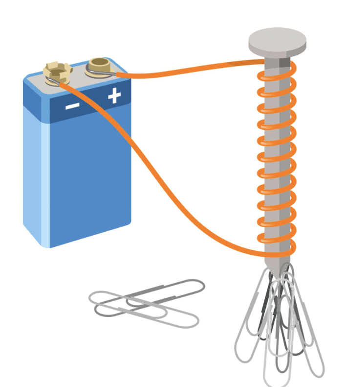
Magnetising a solenoid
A current-carrying coil will create a magnetic field as shown below.
The magnetic field of a solenoid.(Note that the field lines in the centre are truncated to save space, but would form very large loops as mentioned above.)
The wire is usually insulated (often with a tough, transparent and nearly invisible enamel coating for commercial solenoids), but doesn’t have to be. Insulation prevents annoying ‘short circuits’ if the coils touch. At first sight, we see the familiar ‘butterfly field’ pattern, but we also see a very intense magnetic field in the centre of the solenoid,
For a typical air-cored solenoid used in a school laboratory carrying one ampere of current, the magnetic field in the centre would have a strength of about 84 microtesla. This is of the same order as the Earth’s magnetic field (which has a typical value of about 50 microtesla). This is just strong enough to deflect the needle of a magnetic compass placed a few centimetres away and (probably) make iron filings align to show the magnetic field pattern around the solenoid, but not strong enough to attract even a small steel paper clip. For reference, the strength of a typical school bar magnet is about 10 000 microtesla, so our solenoid is over one hundred times weaker than a bar magnet.
However, we can ‘boost’ the magnetic field by adding an iron core. The relative permeability of a material is a measurement of how ‘transparent’ it is to magnetic field lines. The relative permeability of pure iron is about 1500 (no units since it’s relative permeability and we are comparing its magnetic properties with that of empty space). However, the core material used in the school laboratory is more likely to be steel rather than iron, which has a much more modest relative permeability of 100.
So placing a steel nail in the centre of a solenoid boosts its magnetic field strength by a factor of 100 — which would make the solenoid roughly as strong as a typical bar magnet.
But which end is north…?
The N and S-poles of a solenoid can change depending on the direction of current flow and the geometry of the loops.
The typical methods used to identify the N and S poles are shown below.
Methods of locating N and S pole of a solenoid that you should NOT use…
To go in reverse order for no particular reason, I don’t like using the second method because it involves a tricky mental rotation of the plane of view by 90 degrees to imagine the current direction as viewed when looking directly at the ends of the magnet. Most students, understandably in my opinion, find this hard.
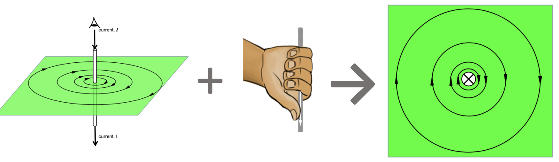
The first method I dislike because it creates confusion with the ‘proper’ right hand grip rule which tells us the direction of the magnetic field lines around a long straight conductor and which I’ve written about before . . .
The right hand grip rule illustrated: the field line curl in the same direction as the finger when the thumb is pointed in the direction of the current.
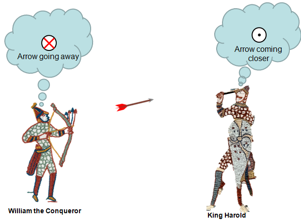
The direction of the current in the last diagram is shown using the ‘dot and cross’ convention which, by a strange coincidence, I have also written about before . . .
If King Harold had been more familiar with the dot and cross notation, history could have turned out very differently…
How a solenoid ‘makes’ its magnetic field . . .
To begin the analysis we imagine the solenoid cut in half: what biologists would call a longitudinal section. Then we show the current directions of each element using the dot and cross convention. Then we consider just two elements, say A and B as shown below.
Continuing this analysis below:
The region inside the solenoid has a very strong and nearly uniform magnetic field. By ‘uniform’ we mean that the field lines are nearly straight and equally spaced meaning that the magnetic field has the same strength at any point.
The region outside the solenoid has a magnetic field which gradually weakens as you move away from the solenoid (indicated by the increased spacing between the field lines); its shape is also nearly identical to the ‘butterfly field’ of a bar magnet as mentioned above.
Since the field lines are emerging from X, we can confidently assert that this is a north-seeking pole, while Y is a south-seeking pole.
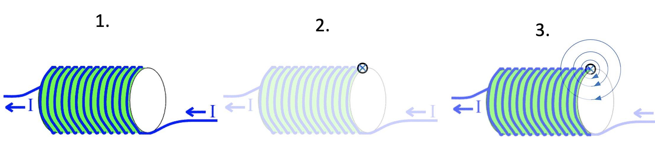
Which end is north, using only the ‘proper’ right hand grip rule…
First, look very carefully at the geometry of current flow (1).
Secondly, isolate one current element, such as the one shown in picture (2) above.
Thirdly, establish the direction of the field lines using the standard right hand grip rule (3).
Since the field lines are heading into this end of the solenoid, we can conclude that the right hand side of this solenoid is, in fact, a south-seeking pole.
In my opinion, this is easier and more reliable than using any of the other alternative methods. I hope that readers that have read this far will (eventually) come to agree.


:format(jpeg):mode_rgb():quality(40)/discogs-images/R-7900735-1451266037-4913.jpeg.jpg)