e=mc2andallthat

A potential divider circuit is, essentially, a circuit where two or more components are arranged in series.

For non-physicists, these types of circuit can sometimes present problems, so in this post I am going to look in detail at the basic physics involved; and I am going to explain them using the CTM or Coulomb Train Model. (You can find the CTM model explained here.)

In the AQA GCSE Physics (and Combined Science) specifications, students are required to know that:

First, let’s look at the basics of describing electric circuits: current, potential difference and resistance.

1.0 Using the CTM to explain current, potential difference and resistance

Pupils tend to start with one concept for electricity in a direct current circuit: a concept labelled ‘current’, or ‘energy’ or ‘electricity’, all interchangeable and having the properties of movement, storability and consumption. Understanding an electrical circuit involves first differentiating the concepts of current, voltage and energy before relating them as a system, in which the energy transfer depends upon current, time and the potential difference of the battery.

The notion of current flowing in the circuit is one which pupils often meet in their introduction to a circuit and, because this relates well with their intuitive notions, this concept becomes the primary concept. (Driver 1994: 124 [italics added])

To my mind, the CTM is an excellent “bridging analogy” that helps students visualise the invisible. It is a stepping stone that provides some concrete representations of abstract quantities. In my opinion, it can help students

1. move away from analysing circuits in terms of just current. (In my experience, even when students use terms like “potential difference”, in their eyes what they call “potential difference” behaves in a remarkably similar way to current e.g. it “flows through” components.)
2. understand the difference between current, potential difference and resistance and how important each one is
3. begin thinking of a circuit as a whole, interconnected system.

1.1 The CTM and electric current

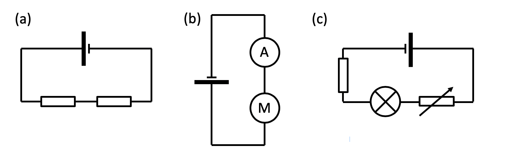
Let’s begin by looking at a very simple circuit: a one ohm resistor connected across a 1 V cell.

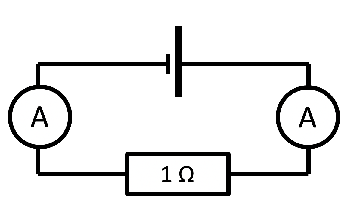
Note that it is a good teaching technique to include two ammeters on either side of the component, although the readings on both will be identical. This is to challenge the perennial misconception that electric current is “used up”. Electric charge, according to our current understanding of the universe, is a conserved quantity like energy in that it cannot be created or destroyed.

The Coulomb Train Model invites us to picture an electric circuit as a flow of positively charged coulombs carrying energy around the circuit in a clockwise fashion as shown below. The coulombs are linked together to form a continuous chain.

The name coulomb is not chosen at random: it is the SI unit of electric charge.

The current in this circuit will be given by I = V / R (equation 18 in the list on p.96 of the AQA spec, if you’re keeping track).

Using the AQA mark scheme-friendly FIFA protocol:

The otherwise inexplicable use of the letter “I” to represent electric current springs from the work André-Marie Ampère (1775–1836) and the French phrase intensité de courant (intensity of current).

From Q = I t (equation 17, p.96), current is a flow of electric charge, since I = Q / t. That is to say, if a charge of 2 coulombs passes (AQA call this a “charge flow”) in 2 seconds, the current will be …

A current of 1 amp is therefore represented on the CTM as 1 coulomb (or truck) passing by each second.

1.2 The CTM and Potential Difference

Potential difference or voltage is essentially the “energy difference” across any two parts of a circuit.

The equation used to define potential difference is not the familiar V = IR but rather the less familiar E = QV (equation 22 in the AQA list) where E is the energy transferred, Q is the charge flow (or the number of coulombs passing by in a certain time) and t is the time in seconds.

Let’s see what this would look like using the CTM:

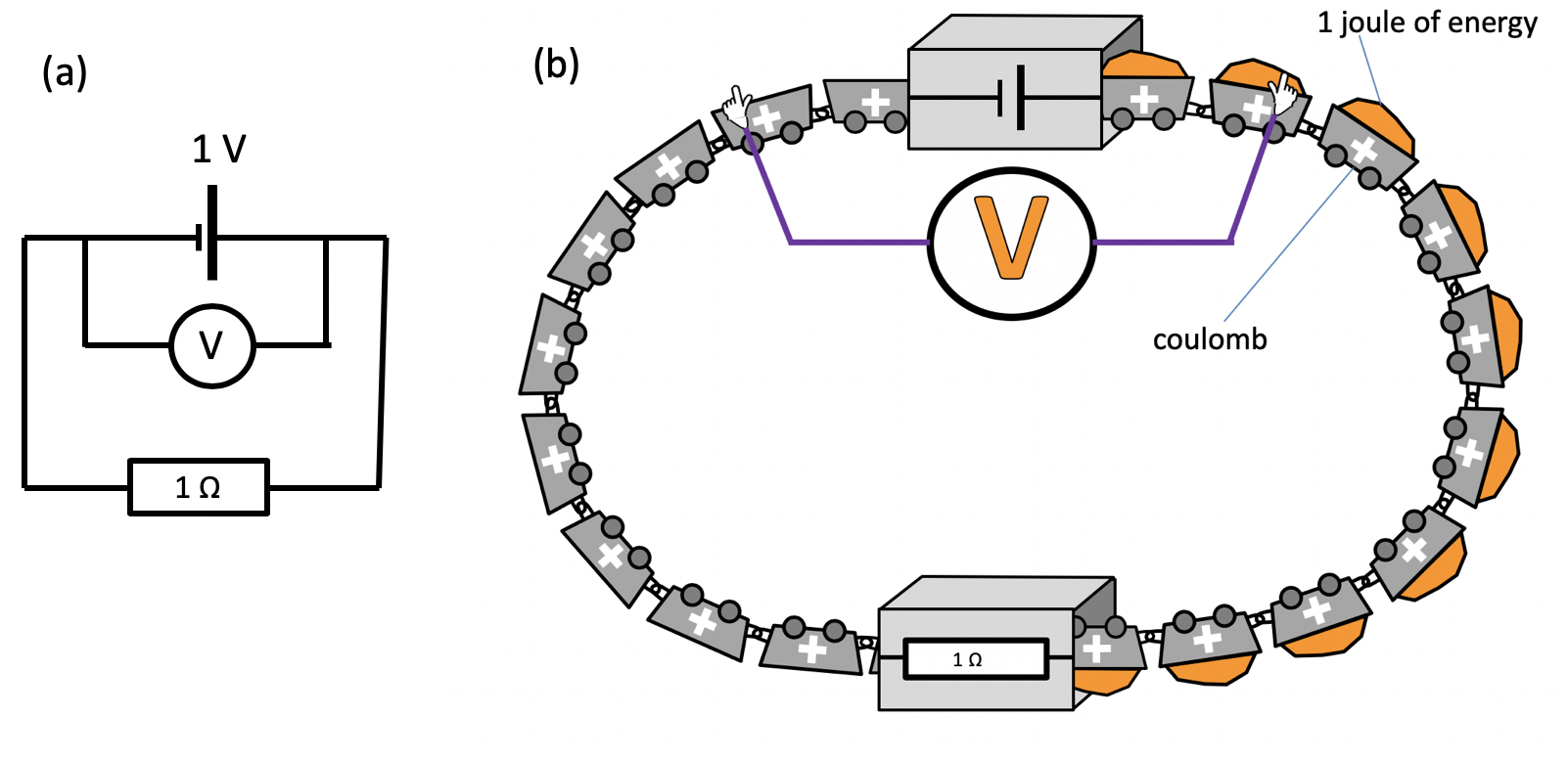
For the circuit shown, the voltmeter reading is 1 volt.

Note that on the CTM representation, one joule of energy is added to each coulomb as it passes through the cell.

If we had a 1.5 V cell then 1.5 joules would be transferred to each coulomb as it passed through, and so on.

If the voltmeter is moved to a different position as shown above, then the reading is 0 volts. This is because the coulombs at the points “sampled” by the voltmeter have the same amount of energy, so there is zero energy difference between them.

In the position shown above, the voltmeter is measuring the potential difference across the resistor. For the circuit shown (assuming negligible resistance in all other parts of the circuit) the potential difference will be 1 V. In other words, each coulomb is losing one joule of energy as it passes through the resistance.

1.3 The CTM and Resistance

In the circuit above, the potential difference across the resistor is 1 V and the current is 1 amp.

Resistance can therefore be thought of as the potential difference required to drive a current of 1 amp through that part of the circuit. It can also be thought of as the energy lost by each coulomb when a current of 1 amp flows through that part of the circuit; or, energy lost per coulomb per amp.

1.4 Summary

On the diagrams below, the coulombs are moving clockwise.

2.0 The CTM applied to a potential divider circuit

A potential divider circuit simply means that at least two resistors are in series so that the potential difference of the cell is shared across the resistors.

2.1 Two identical resistors

Because the two resistors are identical, the 3 V supply is shared equally across both resistors. That is to say, there is a potential difference of 1.5 V across each resistor. But let’s check this by applying V = IR (eq. 18). The total potential difference is 3 V and the total resistance is 1 ohm + 1 ohm = 2 ohms.

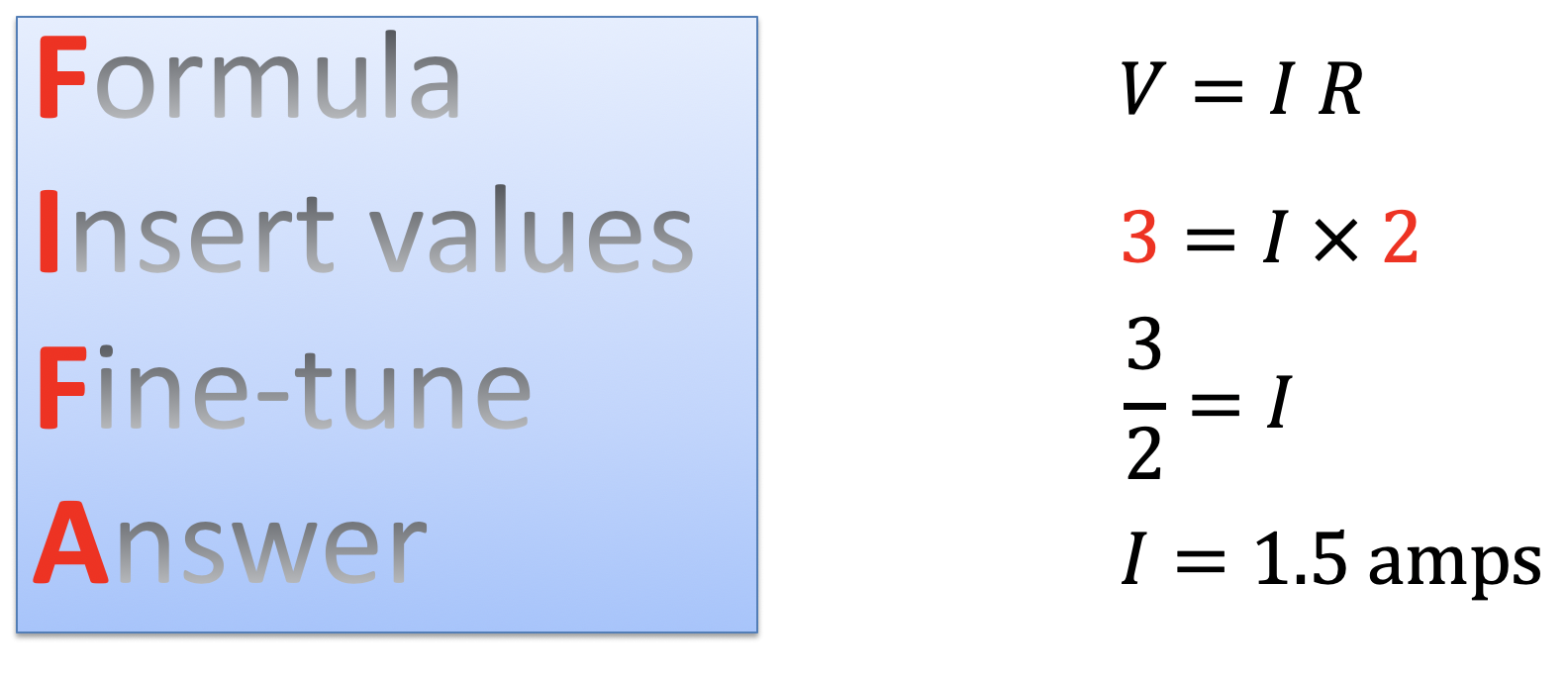
Now let’s use V = IR to check that the potential difference across each separate resistor is indeed half the total supply of 3 V. The resistance of one resistor is one ohm and the current through each one is 1.5 A. So V = 1.5 x 1 = 1.5 V.

But what would happen if we doubled the value of each resistor to 2 ohms?

Well, the current would be smaller: I = V/R = 3/4 = 0.75 amps.

The potential difference across each separate resistor would be V = I R = 0.75 x 2 = 1.5 V

So, the potential difference is always split equally when two identical resistors are placed in series (although, of course, the total resistance and the current will be different depending on the values of the resistors).

2.2a Two non-identical resistors

Let’s consider a circuit with a 2 ohm resistor in series with a 1 ohm resistor.

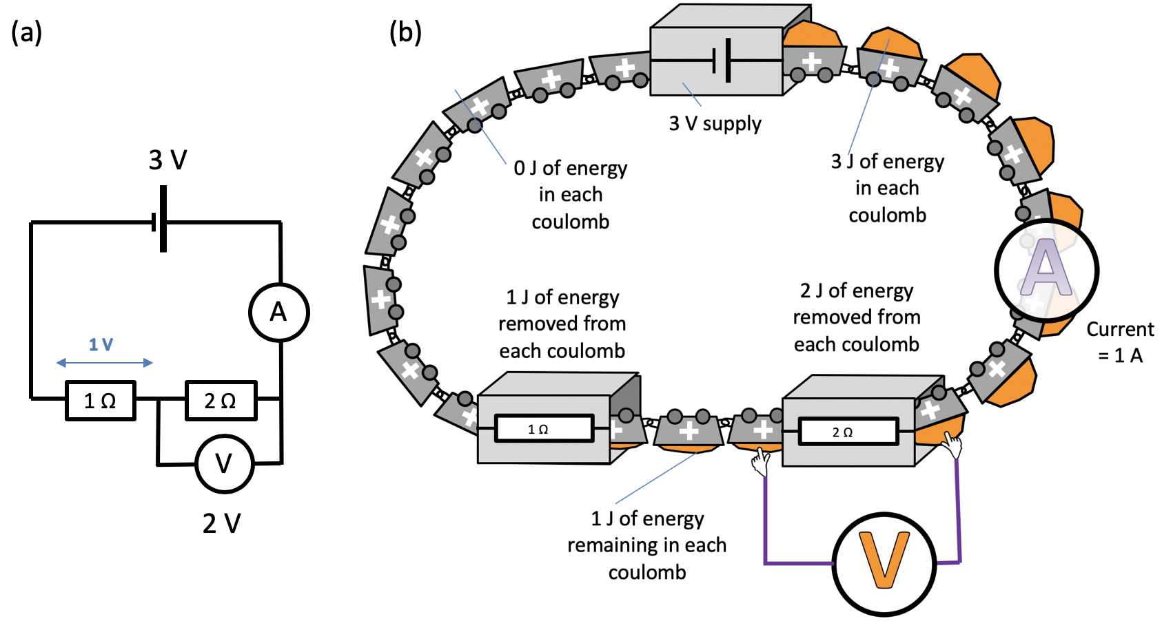
In this circuit, the total resistance is 1 ohm + 2 ohms = 3 ohms. The current flowing through the circuit is I = V / R = 3 / 3 = 1 amp.

So the potential difference across the 2 ohm resistor is V = IR = 1 x 2 = 2 V and the potential difference across the one ohm resistor is V = IR = 1 x 1 = 1 V.

Note that the resistor with the largest value gets the largest “share” of the potential difference.

2.2b Two non-identical resistors (different order)

Now let’s reverse the order of the resistors.

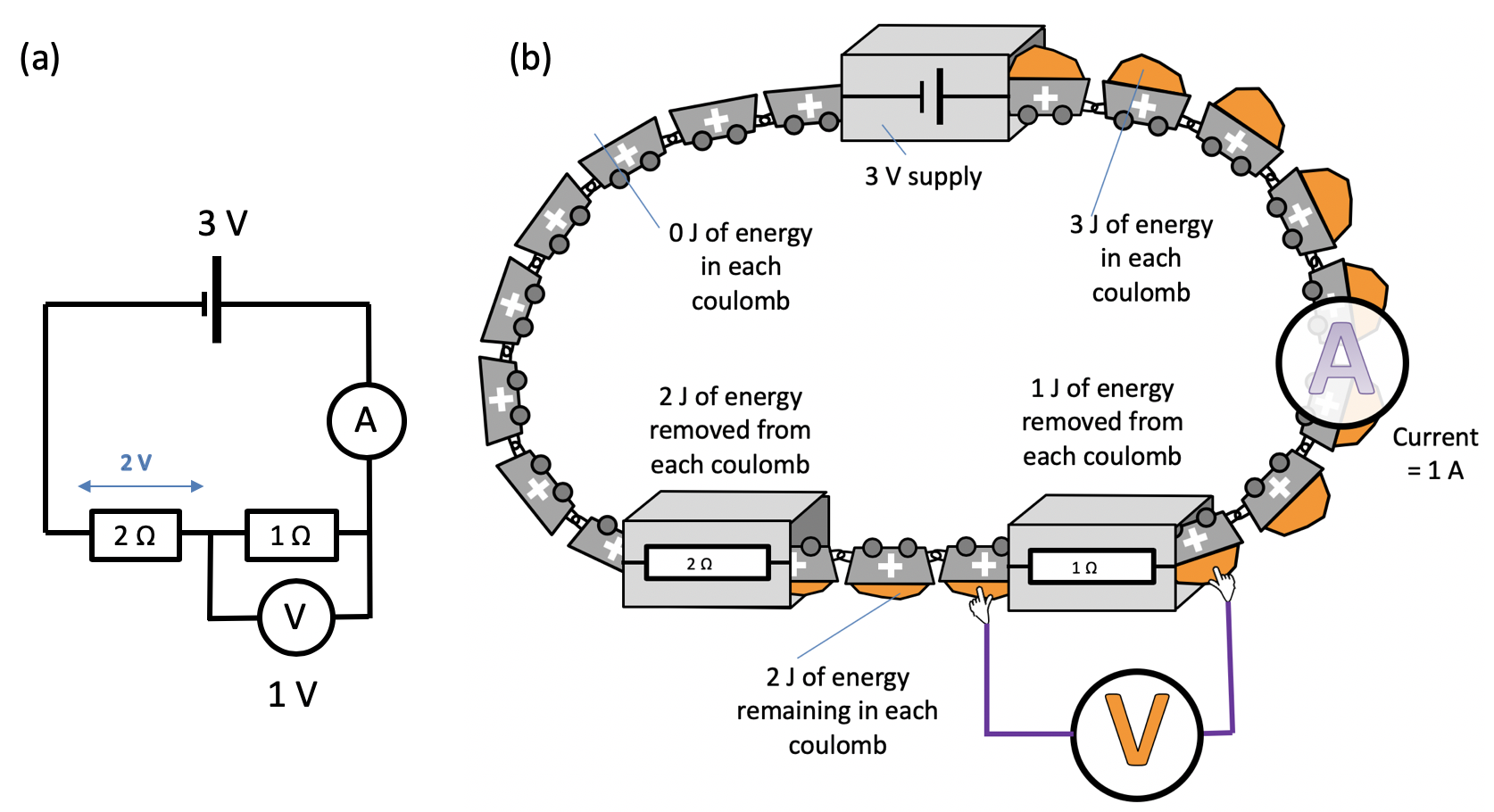
The current remains unchanged because the total resistance of the circuit is still the same.

Note that the largest resistor still gets the largest share of the potential difference, whichever way round the resistors are placed.

2.3 In Defence of the CTM and Donation Models

Many Physics teachers prefer “rope models” to so-called “donation models” like the CTM.

And it is perfectly true that rope models have some good points such as the ability to easily explain AC and a more accurate approximation of what happens when current starts to flow or stops flowing. The difficulty in their use, in my opinion, is that you are using concepts that many students barely understand (e.g. friction to model resistance) to explain how very unfamiliar concepts such as potential difference work. Also, the vagueness of some of the analogs is unhelpful: for example, when we compare potential difference to “push”, are we talking about the net resultant force on the rope or simply the force needed to balance the frictional force and keep it moving at a steady speed?

To my way of thinking, the CTM has the advantage of encouraging quantitative thinking about current, potential difference and resistance almost from the moment of first teaching. Admittedly, it cannot cope with AC — but then again, we model AC as a direct current when we use RMS values. Now admittedly, rope models are far better at picturing what happens in the initial fractions of a second when a current starts to flow after closing a switch. Be that as it may, the CTM comes into its own when we consider the “steady state” of current flow after the initial surge currents.

One of the frequent criticisms (which is usually considered quite damning) of this type of model is “How do the coulombs know how much energy to drop off at each resistor?”

For example, in the diagram above, how do the coulombs “know” to drop off 1 J at the first resistor and 2 J at the second resistor?

The answer is: they don’t. Rather, the energy loss is due to the nature of the resistor: think of a resistor as a tunnel lined with strip curtains. A coulomb loses only a small amount of its excess energy passing through a low value resistor, but a much larger amount passing through a higher value resistor, as modelled below.

FWIW I therefore commend the use of the CTM to all interested parties. 

References

Driver, R., Squires, A., Rushworth, P., & Wood-Robinson, V. (1994). Making sense of secondary science: Research into children’s ideas. Routledge.