Introducing vectors (part 2)

This post suggests some strategies for teaching vectors to 14-16 olds. In part 1 we looked at the idea of combining two vectors into one; that is to say, finding the resultant vector. In this part, we’re going to look at the inverse operation: splitting a single vector into two component vectors.

We’re going to use scale drawing rather than trigonometry since (a) this often leads to a more secure understanding; and (b) it is the expected method in the UK curriculum for 14-16 year olds.

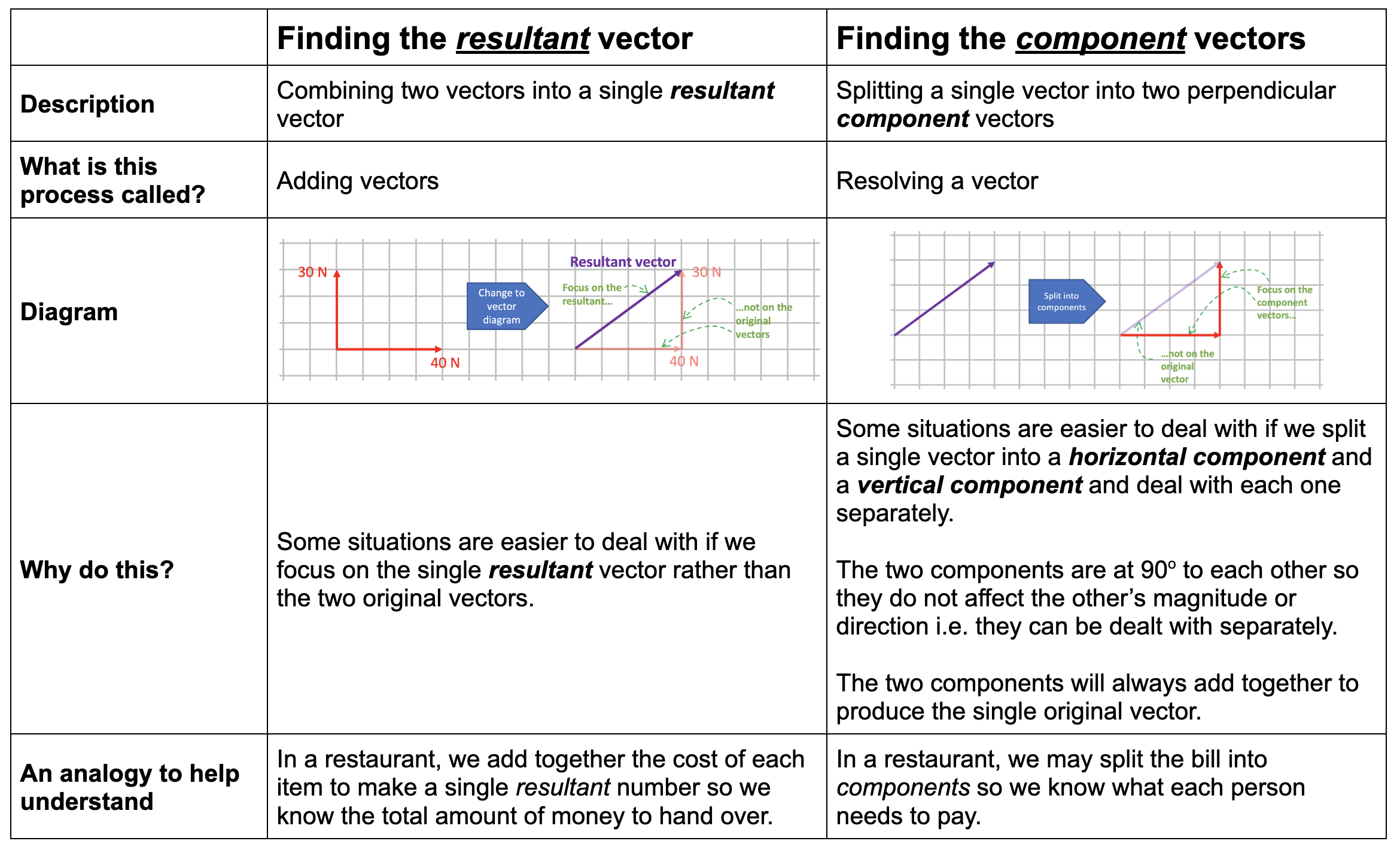
What is a component vector?

A component vector is one of at least two vectors that will combine to give one single original vector. The component vectors are chosen so that they are mutually perpendicular. Because of this, they cannot affect each other’s magnitude and direction and so can be dealt with separately and independently; that is to say, we can choose to consider what effect the vertical component will have on its own without having to worry about what effect the horizontal component will have.

Introducing components as ‘the vector less travelled by’

Two roads diverged in a wood, and I—
I took the one less traveled by,
And that has made all the difference.

Robert Frost, 'The Road Less Travelled'

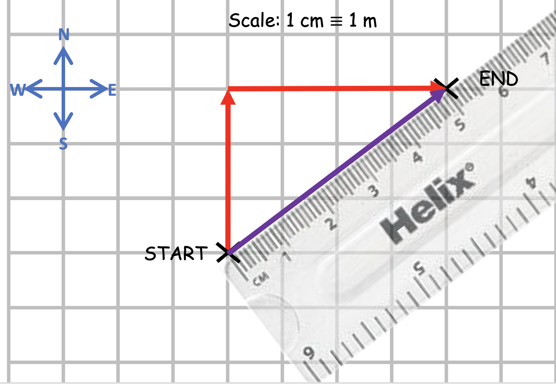
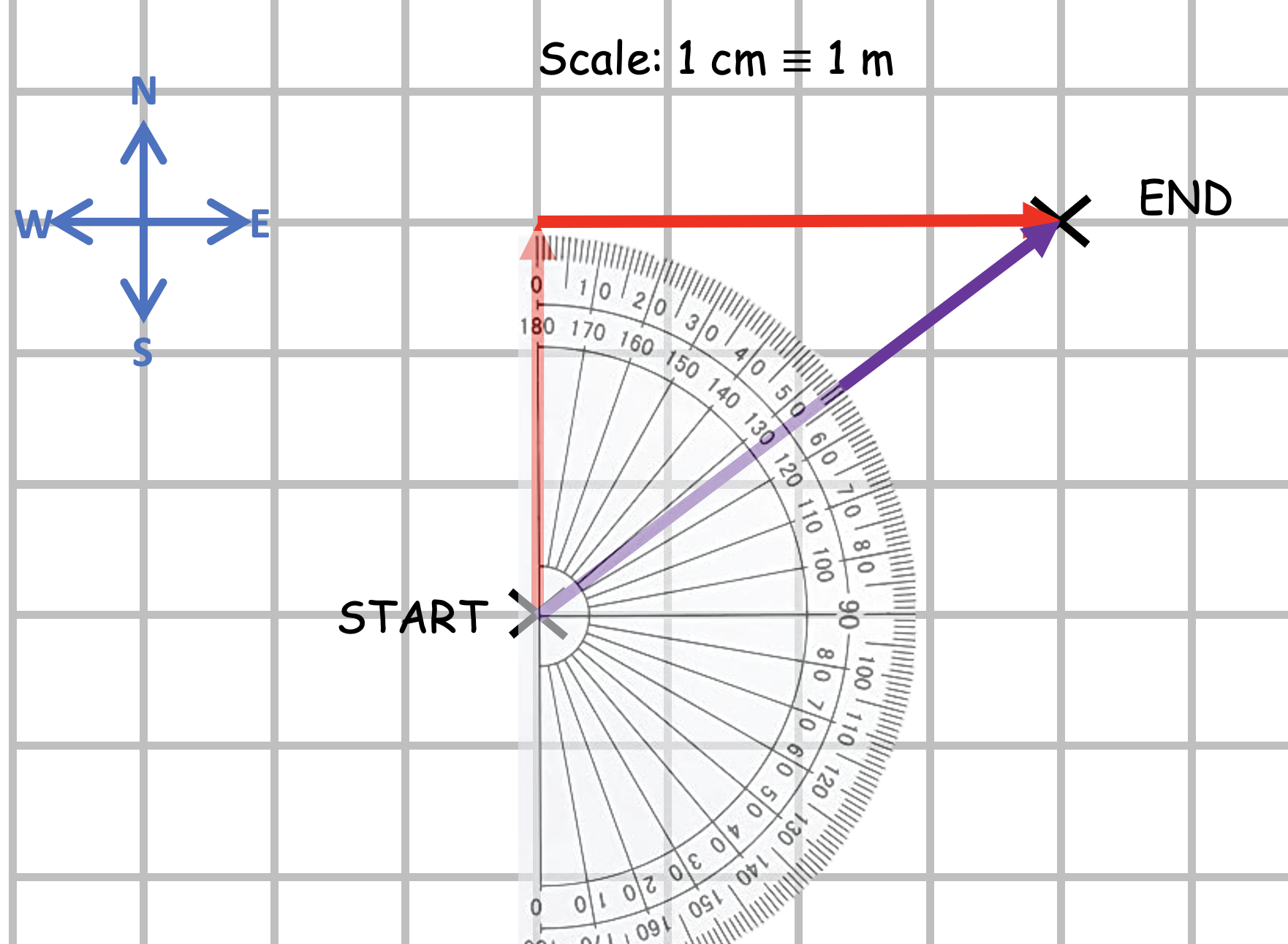
Let’s say we travelled a distance of 13 m from point O to point P on a compass bearing of 067 degrees (bear with me, I’m working with a slightly less familiar Pythagorean 3:4:5 triple here). This could be drawn as a scale diagram as shown below.

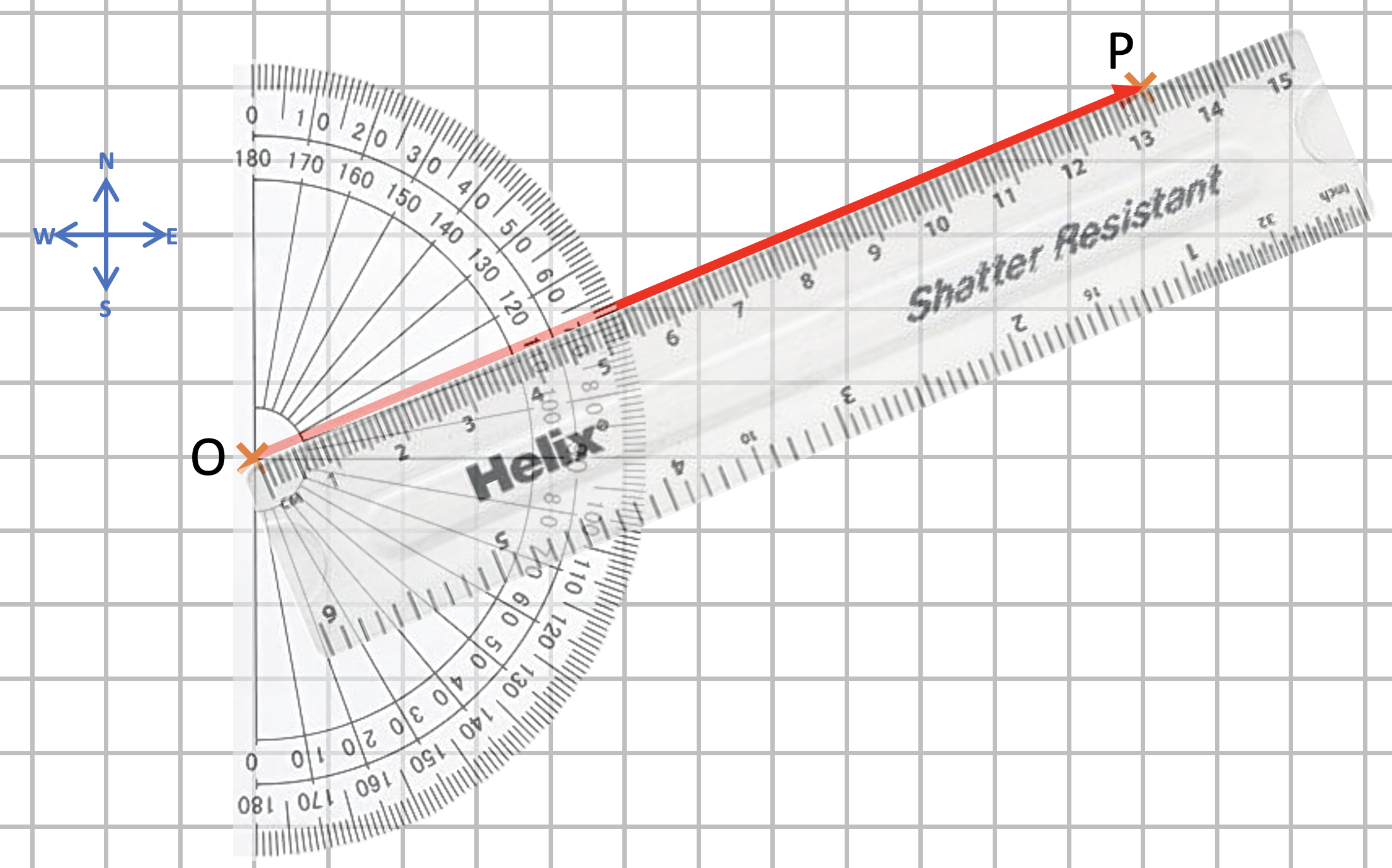
Could we analyse the displacement OP in terms of an eastward displacement and a northward displacement?

We can — as shown below.

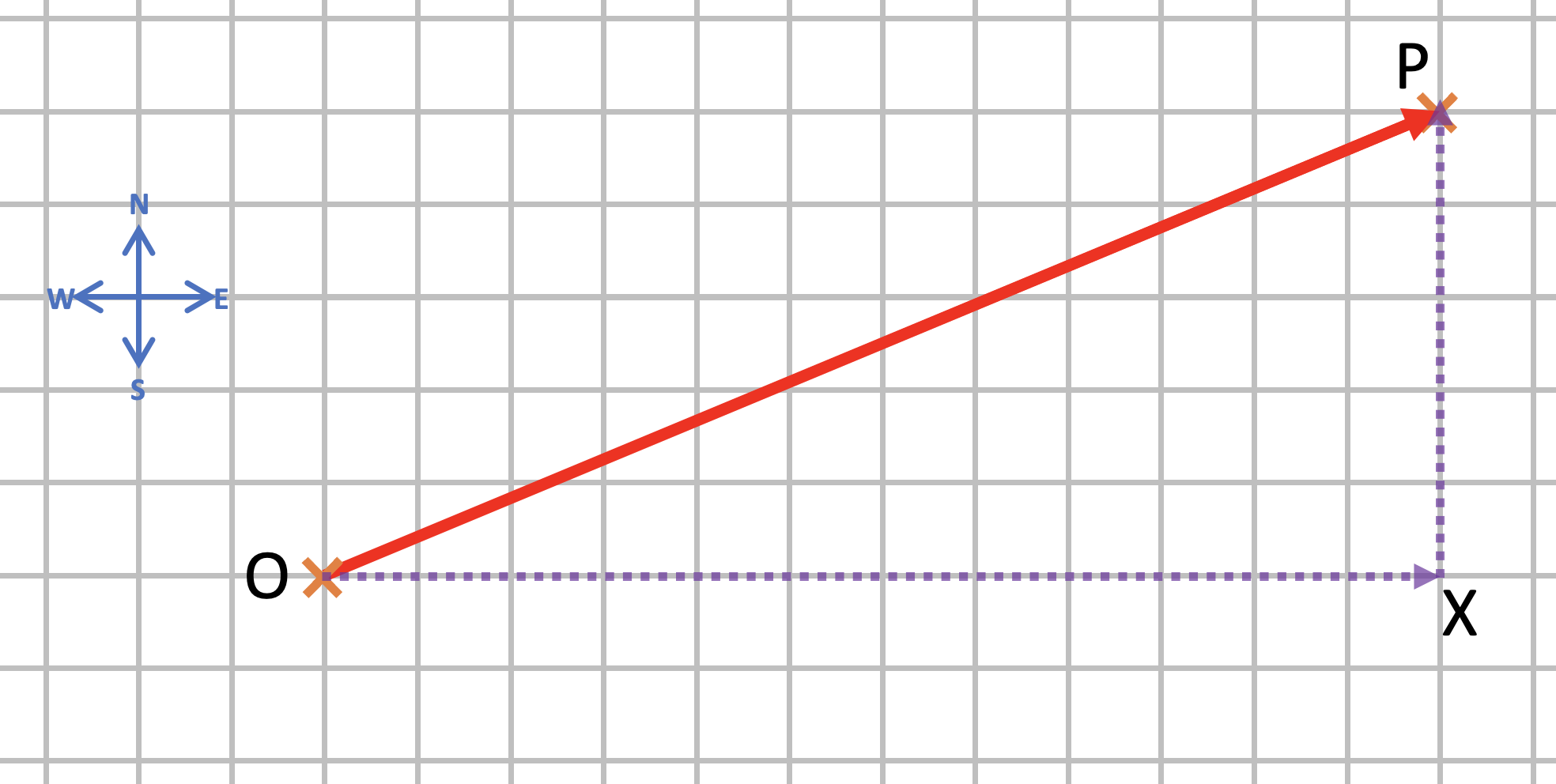
The dotted line OX is the eastward (horizontal on our diagram) component of the displacement OP. It is drawn as a dotted line because it is (literally) the ‘road less travelled’. We did not walk along that road — and that’s why it is drawn as a dotted line — but we could have done.

But let’s say that we had, and that we had stopped when we reached the point marked X. And then we look around, and strike out northwards and walk the (vertical) ‘road less travelled called XP — and we end up at P.

So walking one road less travelled might, indeed, make ‘all the difference’ — but walking two roads less travelled does not.

To rewrite Robert Frost: We took the two roads less travelled by / And that has made NO difference.

But why should we wish to go the ‘long way around’, even if we still end up at P? Because it would allow us to work out the change in longitude and latitude. By moving from O to P we change our longitude by 12 metres and our latitude by 5 metres. (Don’t believe me? Count the squares on the diagram!)

We have resolved the 13 metre distance into two components: one eastward (horizontal) component of 12 metres and one northward component of 5 metres.

Using resolving a vector into components to solve problems

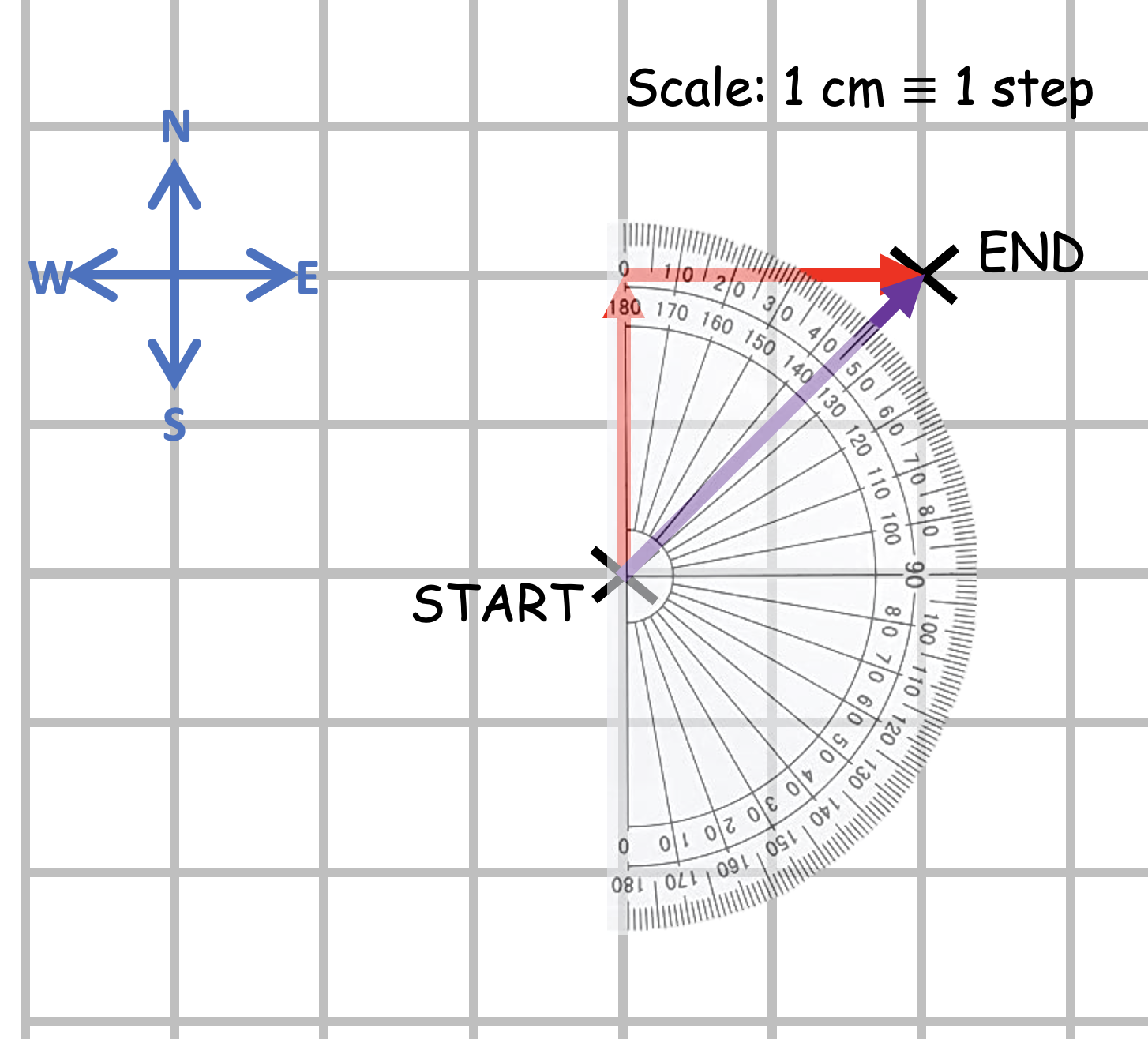
We can use the scale drawing technique outlined above to resolve (‘split’) the 3000 N vector into a horizontal component and a vertical component.

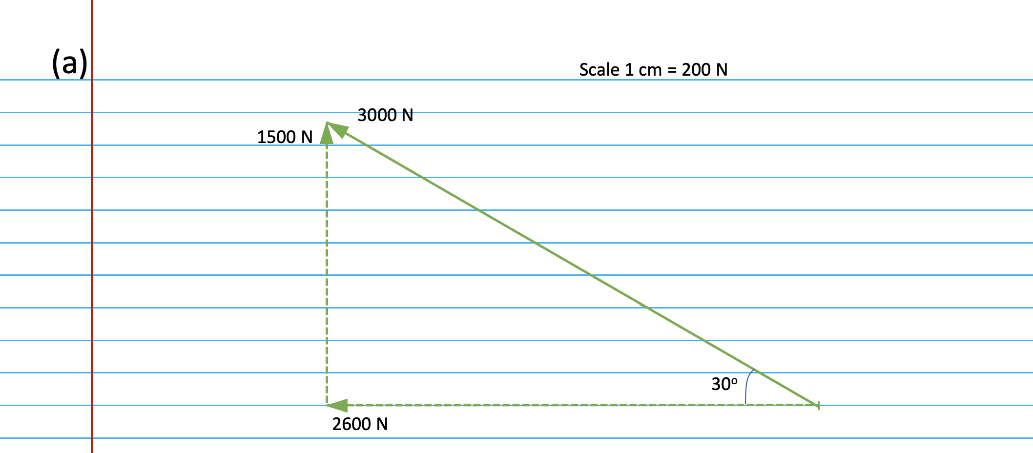
The full solution is shown in sequence on this PowerPoint.

Introducing vectors (part 1)

I think that teaching vectors to 14-16 year olds is a bit like teaching them to play the flute; that is to say, it’s a bit like teaching them to play the flute as presented by Monty Python (!)

Monty Python (1972), ‘How to play the flute’

Part of the trouble is that the definition of a vector is so deceptively and seductively easy: a vector is a quantity that has both magnitude and direction.

There — how difficult can the rest of it be? Sadly, there’s a good deal more to vectors than that, just as there’s much more to playing the flute than ‘moving your fingers up and down the outside'(!)

What follows is a suggested outline teaching schema, with some selected resources.

Resultant vector = total vector: the ‘I’ phase

‘2 + 2 = 4’ is often touted as a statement that is always obviously and self-evidently true. And so it is — arithmetically and for mere scalar quantities. In fact, it would be more precisely rendered as ‘scalar 2 + scalar 2 = scalar 4’.

However, for vector quantities, things are a wee bit different. For vectors, it is better to say that ‘vector 2 + vector 2 = a vector quantity with a magnitude somewhere between 0 and 4’.

For example, if you take two steps north and then a further two steps north then you end up four steps away from where you started. Also, if you take two steps north and then two steps south, then you end up . . . zero steps from where you started.

So much for the ‘zero’ and ‘four’ magnitudes. But where do the ‘inbetween’ values come from?

Simples! Imagine taking two steps north and then two steps east — where would you end up? In other words, what distance and (since we’re talking about vectors) in what direction would you be from your starting point?

This is most easily answered using a scale diagram.

To calculate the vector distance (aka displacement) we draw a line from the Start to the End and measure its length.

The length of the line is 2.8 cm which means that if we walk 2 steps north and 2 steps east then we up a total vector distance of 2.8 steps away from the Start.

But what about direction? Because we are dealing with vector quantities, direction just as important as magnitude. We draw an arrowhead on the purple line to emphasise this.

Students may guess that the direction of the purple ‘resultant’ vector (that is to say, it is the result of adding two vectors) is precisely north-east, but this can be a vague description so let’s use a protractor so that we can find the compass bearing.

And thus we find that the total resultant vector — the result of adding 2 steps north and 2 steps east — is a displacement of 2.8 steps on a compass bearing of 045 degrees.

Resultant vector = total vector: the ‘We’ phase

How would we go about finding the resultant vector if we moved 3 metres north and 4 metres east? If you have access to an interactive whiteboard, you could choose to use this Jamboard for this phase. (One minor inconvenience: you would have to draw the straight lines freehand but you can use the moveable and rotatable ruler and protractor to make measurements ‘live’ with your class.)

We go through a process similar to the one outlined above.

  • What would be a suitable scale?
  • How long should the vertical arrow be?
  • How long should the horizontal arrow be?
  • Where should we place the ‘End’ point?
  • How do we draw the ‘resultant’ vector?
  • What do we mean by ‘resultant vector’?
  • How should we show the direction of the resultant vector?
  • How do we find its length?
  • How do we convert the length of the arrow on the scale diagram into the magnitude of the displacement in real life?

The resultant vector is, of course, 5.0 m at a compass bearing of 053 degrees.

Resultant vector = total vector: the ‘You’ phase

Students can complete the questions on the worksheets which can be printed from the PowerPoint below.

Answers are shown on this second PowerPoint, plus an optional digital ruler and protractor are included on the third slide if you wish to use them.

Enjoy!

Deriving centripetal acceleration

When I was an A-level physics student (many, many years ago, when the world was young LOL) I found the derivation of the centripetal acceleration formula really hard to understand. What follows is a method that I have developed over the years that seems to work well. The PowerPoint is included at the end.

Step 1: consider an object moving on a circular path

Let’s consider an object moving in circular path of radius r at a constant angular speed of ω (omega) radians per second.

The object is moving anticlockwise on the diagram and we show it at two instants which are time t seconds apart. This means that the object has moved an angular distance of ωt radians.

Step 2: consider the linear velocities of the object at these times

The linear velocity is the speed in metres per second and acts at a tangent to the circle, making a right angle with the radius of the circle. We have called the first velocity v1 and the second velocity at the later time v2.

Since the object is moving at a constant angular speed ω and is a fixed radius r from the centre of the circle, the magnitudes of both velocities will be constant and will be given by v = ωr.

Although the magnitude of the linear velocity has not changed, its direction most certainly has. Since acceleration is defined as the change in velocity divided by time, this means that the object has undergone acceleration since velocity is a vector quantity and a change in direction counts as a change, even without a change in magnitude.

Step 3a: Draw a vector diagram of the velocities

We have simply extracted v1 and v2 from the original diagram and placed them nose-to-tail. We have kept their magnitude and direction unchanged during this process.

Step 3b: close the vector diagram to find the resultant

The dark blue arrow is the result of adding v1 and v2. It is not a useful operation in this case because we are interested in the change in velocity not the sum of the velocities, so we will stop there and go back to the drawing board.

Step 3c switch the direction of velocity v1

Since we are interested in the change in velocity, let’s flip the direction of v1 so that it going in the opposite direction. Since it is opposite to v1, we can now call this -v1.

It is preferable to flip v1 rather than v2 since for a change in velocity we typically subtract the initial velocity from the final velocity; that is to say, change in velocity = v2 – v1.

Step 3d: Put the vectors v2 and (-v1) nose-to-tail

Step 3e: close the vector diagram to find the result of adding v2 and (-v1)

The purple arrow shows the result of adding v2 + (-v1); in other words, the purple arrow shows the change in velocity between v1 and v2 due to the change in direction (notwithstanding the fact that the magnitude of both velocities is unchanged).

It is also worth mentioning that that the direction of the purple (v2v1) arrow is in the opposite direction to the radius of the circle: in other words, the change in velocity is directed towards the centre of the circle.

Step 4: Find the angle between v2 and (-v1)

The angle between v2 and (-v1) will be ωt radians.

Step 5: Use the small angle approximation to represent v2-v1 as the arc of a circle

If we assume that ωt is a small angle, then the line representing v2-v1 can be replaced by the arc c of a circle of radius v (where v is the magnitude of the vectors v1 and v2 and v=ωr).

We can then use the familiar relationship that the angle θ (in radians) subtended at the centre of a circle θ = arc length / radius. This lets express the arc length c in terms of ω, t and r.

And finally, we can use the acceleration = change in velocity / time relationship to derive the formula for centripetal acceleration we a = ω2r.


Well, that’s how I would do it. If you would like to use this method or adapt it for your students, then the PowerPoint is attached.

Please Like or leave a comment if you find this useful 🙂