In this post, we will look at understanding potential difference (or voltage) using the Coulomb Train Model.
This is part 2 of a continuing series. You can read part 1 here.
The Coulomb Train Model (CTM) is a helpful model for both explaining and predicting the behaviour of real electric circuits which I think is suitable for use with KS3 and KS4 students (that’s 11-16 year olds for non-UK educators).
To summarise what has been discussed so far:
Modelling potential difference using the CTM
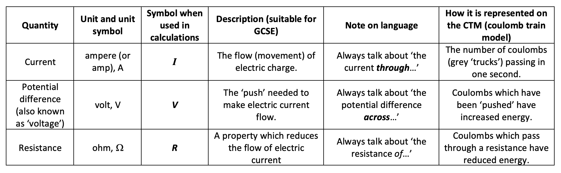
Potential difference is the ‘push’ needed to make electric charge move around a closed circuit. On the CTM, we can represent the ‘push’ as a gain in the energy of the coulomb. (This is consistent with the actual definition of the volt V = E/Q, where one volt is a change in energy of one joule per coulomb.)
How can we observe this gain in energy? Simple, we use a voltmeter.

On the CTM, this would look like this:

What the voltmeter does is compare the energy contained by two coulombs: one at A and the other at B. The coulombs at B, having passed through the 1.5 V cell, each have 1.5 joules of energy more than than the coulombs at A. This means that the voltmeter in this position reads 1.5 volts. We would say that the potential difference across the cell is 1.5 V. (Try and avoid talking about the potential difference ‘through’ or ‘of’ any part of the circuit.)
More potential difference measurements using the CTM
Let’s move the voltmeter to a different position.

On the CTM, this would look like this:

Let’s make the very reasonable assumption that the connecting wires have zero resistance. This would mean that the coulombs at C have 1.5 joules of energy and that the coulombs at D have 1.5 joules of energy. They have not lost any energy since they have not passed through any part of the circuit that actually has a resistance. The voltmeter would therefore read 0 volts since it cannot detect any energy difference.
Now let’s move the voltmeter one last time.

On the CTM, this would look like this:

Notice that the coulombs at F have 1.5 fewer joules than the coulombs at E. The coulombs transfer 1.5 joules of energy to the bulb because the bulb has a resistance.
Any part of the circuit that has non-zero resistance will ‘rob’ coulombs of their energy. On this very simple model, we assume that only the bulb has a resistance and so only the bulb will ‘push back’ against the movement of the coulombs and cost them energy.
Also on this simple model, the potential difference across the bulb is identical to the potential difference across the cell — but this is not always the case. For example, if the wires had a small but non-negligible resistance and if the cell had an internal resistance, but these would only come into play at A-level.
The bulb is shown as ‘flashing’ on the CTM to provide a visual cue to help students mentally model the transfer of energy from the coulombs to the bulb. In reality, instead of just one coulomb transferring a largish ‘chunk’ of energy, there would be approximately 1.25 billion billion electrons continuously transferring a tiny fraction of this energy over the course of one second (assuming a d.c. current of 0.2 amps) so we wouldn’t see the bulb ‘flash’ in reality.
How do the coulombs ‘know’ how much energy to drop off?
This section is probably more of interest to specialist physics teachers, but all are welcome.
One frequent criticism of donation models like the CTM is how do the coulombs ‘know’ to drop off all their energy at the bulb?
The response to this, of course, is that they don’t. This criticism is an artefact of an (arguably) over-simplified model whereby we assume that only the bulb has resistance. The energy carried by the coulombs according to this model could be shown as a sketch graph, and let’s be honest it does look a little dodgy…

But, more accurately, of course, the energy loss is a process rather than an event. And the connecting wires actually have a small resistance. This leads to this graph:

Realistically speaking, the coulombs don’t lose all their energy passing through the bulb: they merely lose most of their energy here due to the process of passing through a high resistance part of the circuit.
In part 3 of this series, we’ll look at how resistance can be modelled using the CTM.
You can read part 3 here.


