Part one: general principles
He knew all the tricks: dramatic irony, metaphor, pathos, puns, parody, litotes* and . . . satire. He was vicious.
Monty Python, The Tale of the Pirhana Brothers
As we all know, students really struggle with questions in science exams which require answers written ‘at paragraph length’ (dread words!). What follows are some tips that I have found useful when coaching students to improve performance.
Many teachers of English enjoy great success with acronyms such as PEEL (Point. Example. Explain. Link). However, I think these have limited applicability in Science as the required output of extended writing questions (EWQs) varies too much for even a loose one-size-fits-all approach.
What I encourage students to do is:
1. Write in bullet points
The bullet points (BPs) should be short but fully grammatical sentences (and not single words or part sentences).
The reason for this is twofold:
- Focus: it stops an attempted answer spiralling out of control. Without organising my answer using BPs, I find myself running out of space. I start with the best of intentions but realise, as I fill in the last remaining line of the allocated space, that I haven’t reached the end of the first sentence yet!!!
- Organisation: it discourages students from repeating the same thing again and again. I have sometimes marked extended writing answers that repeat the same point multiple times. Yes, they have filled the space and yes, they have written in complete sentences. But there is no additional information except the first section rewritten using different words!
2. Use correct scientific vocabulary
Students often make the incorrect assumption that ‘Explain‘ means ‘Explain to a non-specialist using jargon-free everyday language‘.
In fact nothing could be further from the truth. The expectation of EWQs in general is that students should be able to communicate to a scientist-peer using technical language appropriate for GCSE or A-level.
Partly, this misconception is our own fault. When students ask for an explanation from their teachers, we often — with the best of intentions! — try to express it in non-threatening, jargon-free language.
This is the model that many students follow when responding to EWQs. For example, I remember groaning in frustration when marking an A-level Physics script where the student has repeatedly written the word ‘move’ when the terms ‘accelerate’ or ‘constant velocity’ would have communicated her understanding with far more clarity.
In Science, what is often derided as ‘jargon’ isn’t an actual barrier to understanding. In truth, a shared, specialist language is an essential pathway to concision and clarity and a guard-rail against inadvertent miscommunication.
3. Write as many BPs as there are marks
For example, students should aim to write 3 BPs in response to a 3-mark EWQ.
4. Read all your BPs. Taken as a whole — do they *answer* the damn question?
If yes, move on. If no, then add another BP.
Part two: modelling the EWQ response-process
‘What does “quantum” mean, anyway?’
‘It means “add another nought.”‘
Terry Pratchett, Pyramids
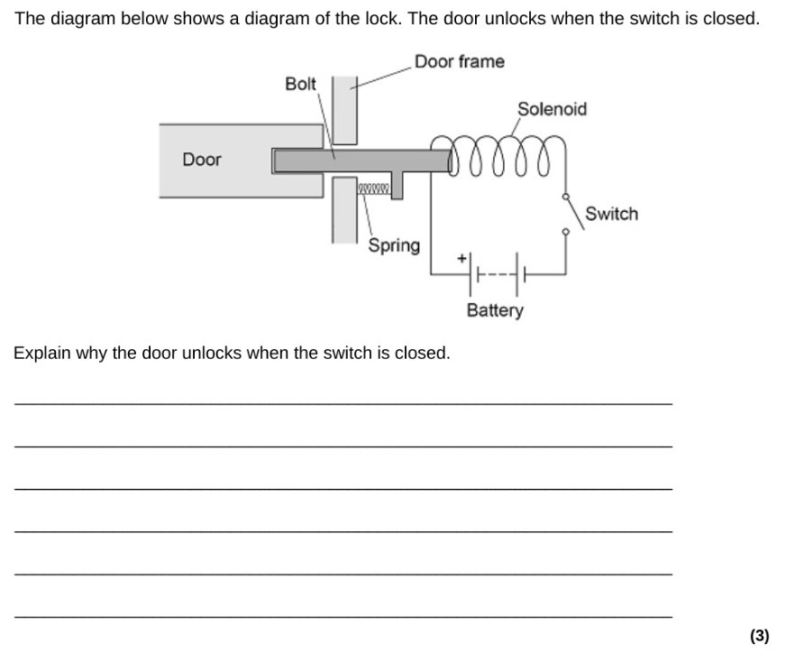
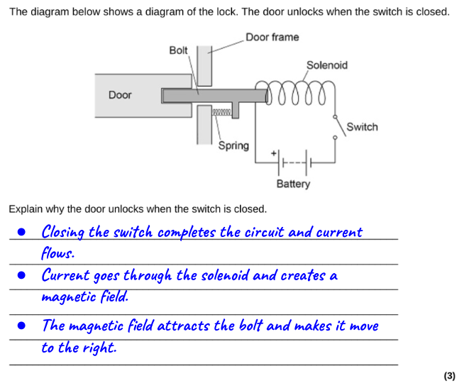
This EWQ has 3 marks, so we should aim for 3 BPs.
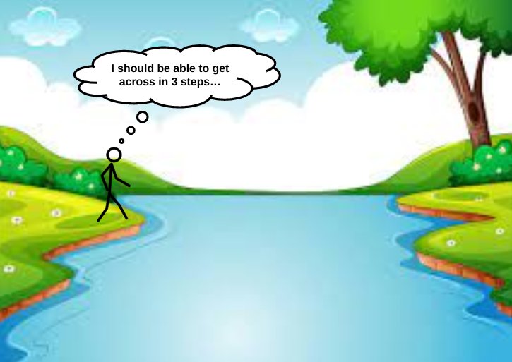
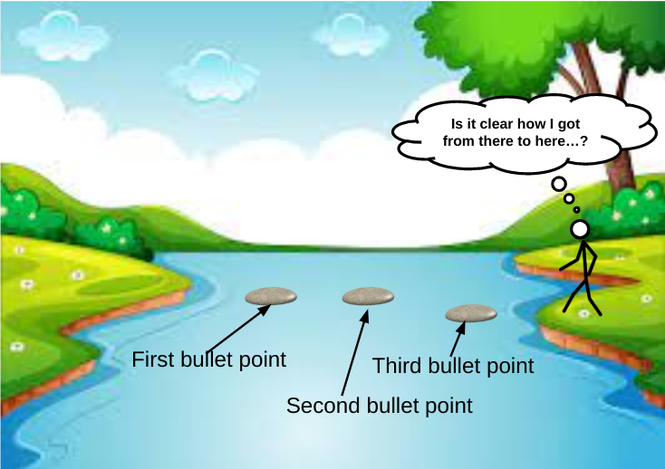
I use the analogy of crossing a river using stepping stones. One stepping stone won’t be enough but three will let us get across — hopefully without us getting our feet wet.
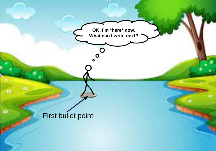
Let’s write our first BP. I suggest that students begin by stating what they may think is obvious.
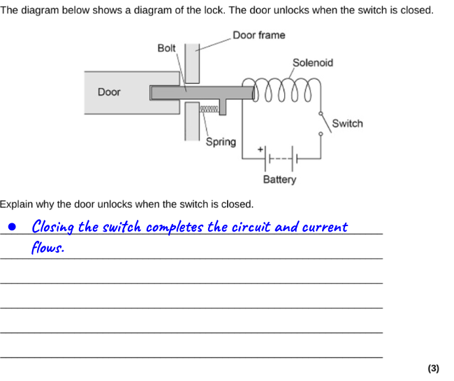
Next, we think about what we could write as our second BP. But — and this is essential! — we consider it from the vantage point of our first BP.
Our second BP is the next-most-obvious-BP: what happens to the solenoid when an electric current goes through it? Remember that we are supposed to use technical language, so we will call a solenoid a solenoid, so to speak.

Next, we consider what to write for our third (and maybe final) BP. Again, we should be thinking of this from the viewpoint of what we have already written.

Finally, and this point is not to be missed, we should look back at all the BPs we have written and ask ourselves the all-important ‘Have I actually answered the question that was asked originally?‘
In this case, the answer is YES, we have explained why the door unlocks when the switch is closed.
This means that we can stop here and move on to the next question.
*Litotes (LIE-tote-ees): an ironic understatement in which an affirmative is expressed as a negative e.g. I won’t be sorry to get to the end of this not-at-all-overlong blog post.