Most of us are only too familiar with the mordant truth of Shakespeare’s observation that “Old men forget, yet all shall be forgot”. In fact, things are generally even worse than the Bard suggests: everyone forgets, all the time.
In time, all shall indeed be forgot.
This was established experimentally by Hermann Ebbinghaus in 1880. The graph below shows Ebbinghaus’ original results with some more recent replications (from Murre and Dros 2015).
However, there is a workaround or “hack” that allows us to beat the Ebbinghaus curve of forgetfulness.
The Power of Review
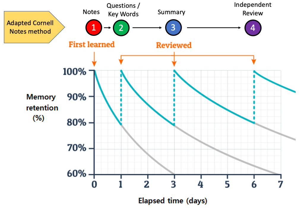
If the content is reviewed at regular intervals, not only do we remember more but the review process also slows down the rate at which knowledge decays.
Cornell notes as a structure for regular review
‘Cornell notes’ is a two column note-taking system developed by Cornell University Professor of Education Walter Pauk (1974). (See also this link.)
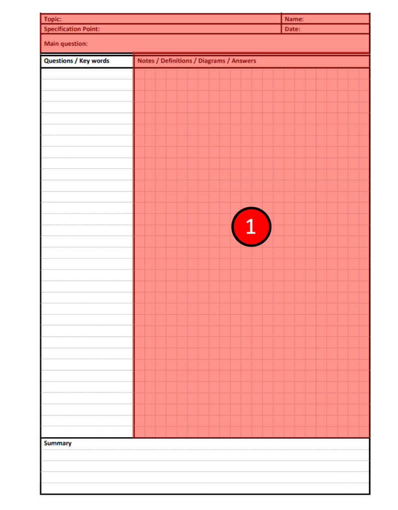
I developed its use in Physics classes with a mind to defeating the Ebbinghaus forgetting curve using this template (click on the link to download a blank printable pdf version).
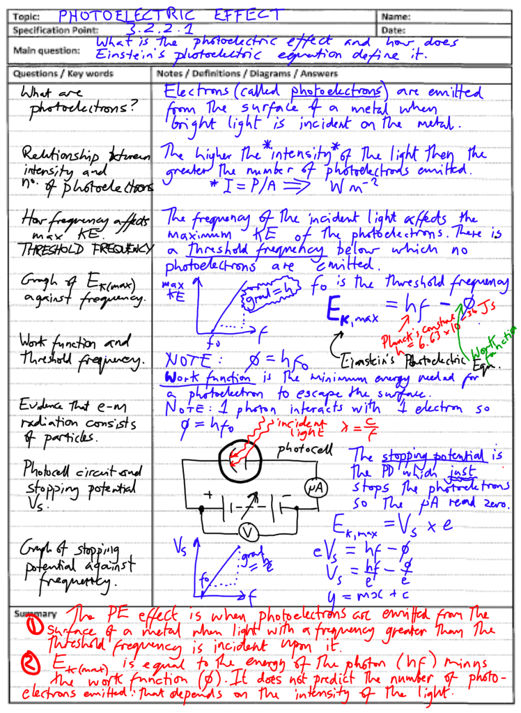
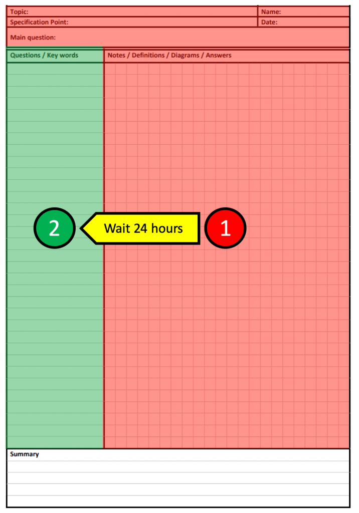
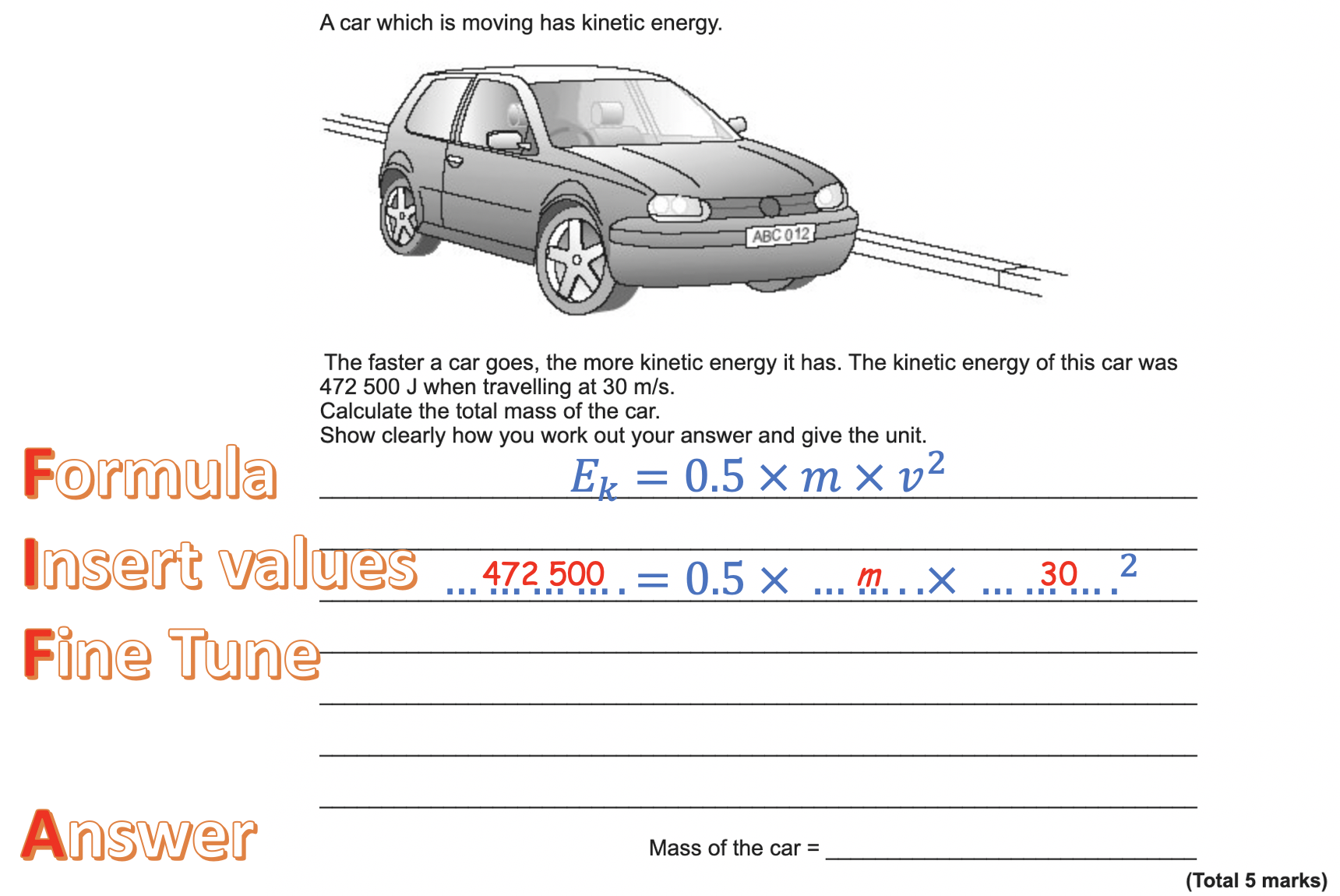
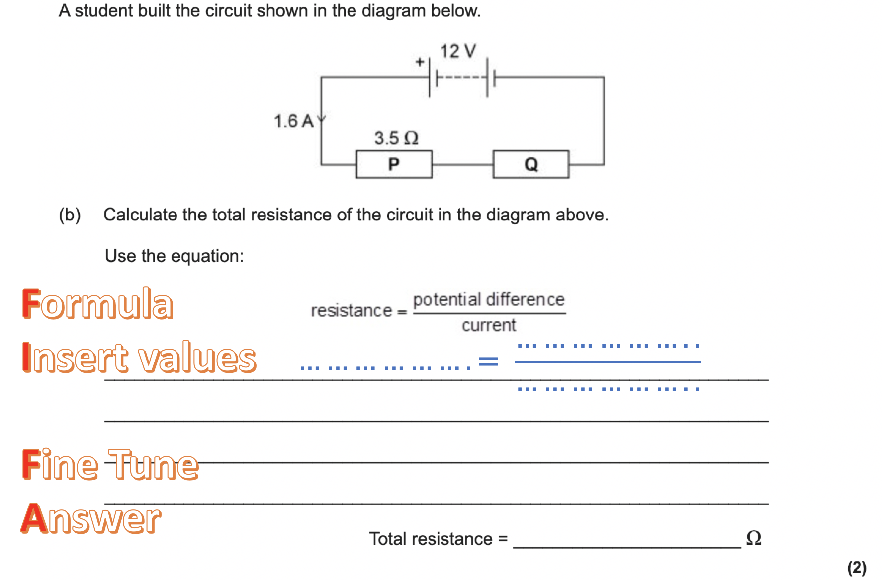
Step 1 Students write notes
In the lesson, students complete the sections highlighted in red but they should leave the other sections blank. This can be a bit of struggle with some students, but is actually a vital part of the process.
Then the students wait 24 hours.
The first couple of times you try this with a class, it might be worth insisting that all students hand in their incomplete Cornell notes at this point just to make sure they follow the process correctly. As students learn to appreciate the effectiveness of the process, you can trust them to follow it without taking control of their work (hopefully!)
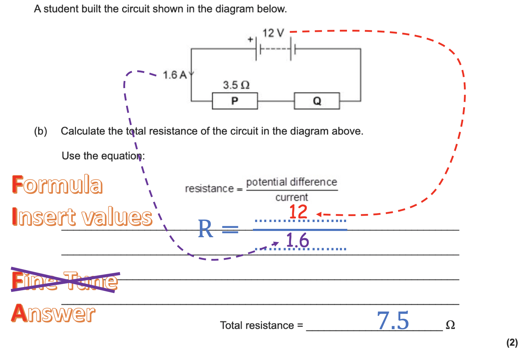
Step 2 Students complete the Questions / Key Words section
After a pause of 24 hours, students then complete the section highlighted in green. Of course, they have to thoroughly review and think hard about the material in the notes section to do this, and in Daniel Willingham’s resonant phrase: “Memory is the residue of thought.”
Then, wait a further 48 hours. (Again, the first couple of times you do this with a class, you may want to take in the incomplete Cornell notes to make sure the process is followed correctly: many students seem to find it impossible to “let it be”!)
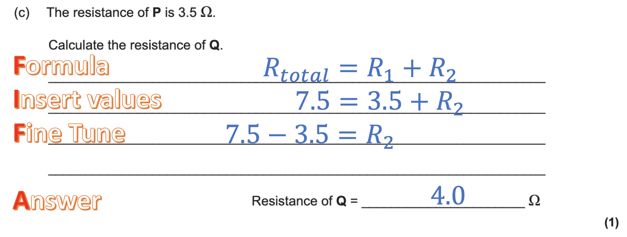
Step 3 Students complete the summary section
48 hours after completing the Questions / Key Words section, students complete the Summary section.
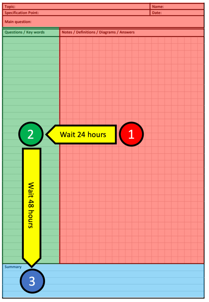
Students often find writing the Summary the hardest part of the process and usually need the most support with this section. The limited space forces concision and an intense focus on the most important concepts — which, of course, is no bad thing in itself!
As an addition to step 3 and following Cho (2011), writing a Reflection on the back of the Cornell notes sheet can be useful to encourage retention. The Reflection is intended to elicit or memorialise an emotional reaction to the content. The context of this could be “Big Picture”, professional, historical or personal.
Students are encouraged to select one context and write something that has emotional resonance for them. Examples relevant to the photoelectric effect (see above) might be:
- “Big picture”: The photoelectric effect is the basis of all light detection technology. Without the science of the photoelectric effect, the fibre optic data networks on which our interconnected society depends would be not only impossible but unthinkable.
- Professional: As an electronic engineer, I would use the photoelectric effect to design super-sensitive electronic cameras that can be used with large aperture telescopes to build up — photon by photon — images of galaxies that are so distant that their light left them four and a half billion years before the Sun formed.
- Historical: Einstein’s 1905 paper on the photoelectric effect was one of the trio of papers published in his “Annus Miriablis” (“Miracle Year”). In the other two he outlined the theory of Special Relativity and used Brownian motion to prove the existence of atoms. Historians of science say that any one of the three would have been enough to secure his reputation as one of the most important physicists of the 20th Century!
- Personal: I thought this was one of the most mathematically challenging topics that we have covered so far in Physics. I am really pleased that I can successfully handle the algebra but also have a good understanding of the physical meaning of all the terms.
Step 4 Independent Review
This can be as simple as covering the red section 1 with a piece of paper and using the Questions and Key Words section as a cue to recall the hidden content.
Conclusion
This was run as a pilot project in Y12 with A-level Physics students. In Y13, they were taught by different teachers who did not use the adapted system. About one quarter of the students who had been taught the process were still using it for Y13 revision and were enthusiastic about how much they felt it boosted their recall of content and understanding.
Some research (e.g. Ahmad 2019) suggests learning gains for students who use the traditional (non-adapted) Cornell notes system. Interestingly, Jacobs (2008) suggests a large improvement in “higher level question” scores for Cornell notes students (again, not the adapted Cornell notes version outlined above).
References
Ahmad, S. Z. (2019). Impact of Cornell Notes vs. REAP on EFL Secondary School Students’ Critical Reading Skills. International Education Studies, 12(10), 60-74.
Cho, J. (2011). Improving science learning through using interactive science notebook (ISN). In P. Gouzouasis (Ed.), Pedagogy in a new tonality (pp. 149-166). Rotterdam, the Netherlands: Sense Publishers. https://doi.org/10.1007/978-94-6091-669-4_10
Chun, B. A., & Heo, H. J. (2018). The effect of flipped learning on academic performance as an innovative method for overcoming Ebbinghaus’ forgetting curve. In Proceedings of the 6th International Conference on Information and Education Technology (pp. 56-60).
Jacobs, K. (2008). A comparison of two note taking methods in a secondary English classroom. Proceedings of the 4th Annual GRASP Symposium, Wichita State University, 2008 (pp. 119-120).
Murre, J. M., & Dros, J. (2015). Replication and analysis of Ebbinghaus’ forgetting curve. PloS one, 10(7), e0120644.
Pauk, W. (1974). How to study in college. Boston: Houghton Mifflin.


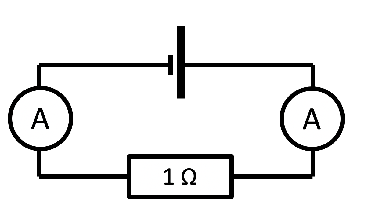


 Because the two resistors are identical, the 3 V supply is shared equally across both resistors. That is to say, there is a potential difference of 1.5 V across each resistor. But let’s check this by applying V = IR (eq. 18). The total potential difference is 3 V and the total resistance is 1 ohm + 1 ohm = 2 ohms.
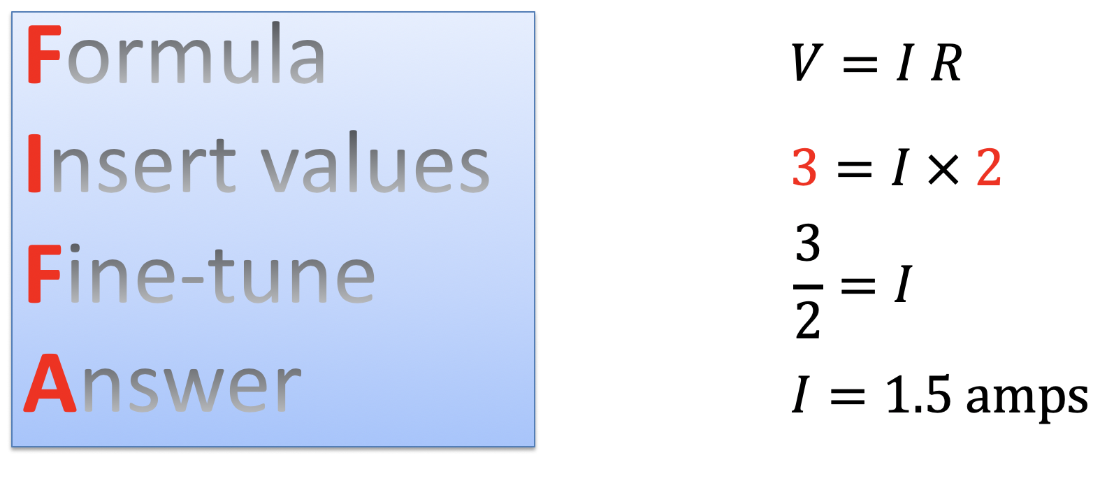

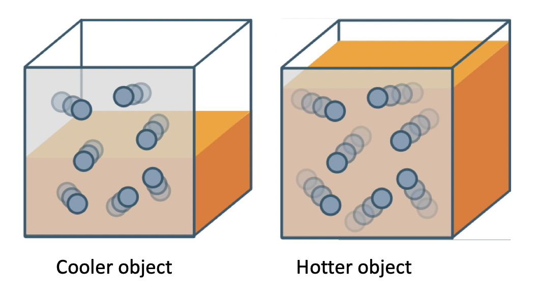
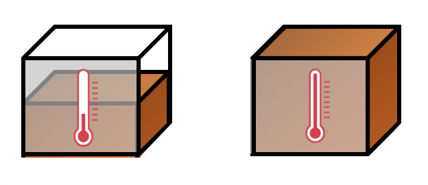
 The enojis for thermal energy stores (as suggested by the