The Coulomb Train Model Revisited (Part 1)

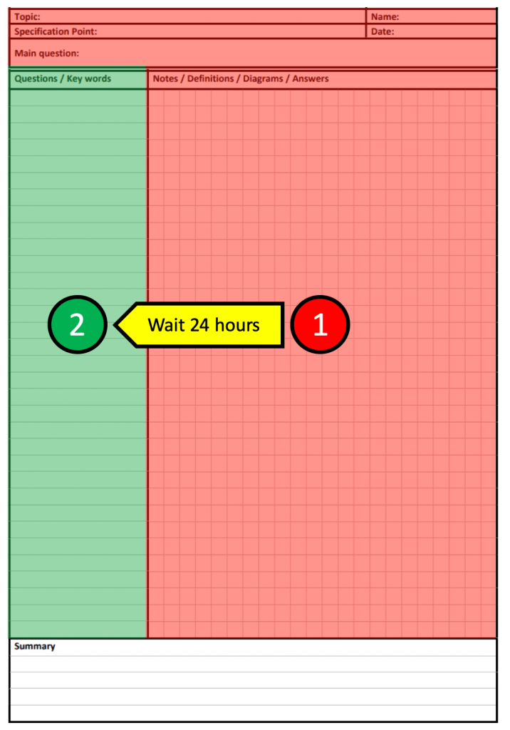
The Coulomb Train Model (CTM) is a helpful model for both explaining and predicting the behaviour of real electric circuits which I think is suitable for use with KS3 and KS4 students (that’s 11-16 year olds for non-UK educators).

I have written about it before (see here and here) but I have recently been experimenting with animated versions of the original diagrams.

Essentially, the CTM is a donation model akin to the famous ‘bread and bakery van’ or even the ‘penguins and ski lift’ models, but to my mind it has some major advantages over these:

  • The trucks (‘coulombs’) in the CTM are linked in a continuous chain. If one ‘coulomb’ stops then they all stop. This helps students grasp why a break anywhere in a circuit will stop all current.
  • The CTM presents a simplified but still quantitatively accurate picture of otherwise abstract entities such as coulombs and energy rather than the more whimsical ‘bread van’ = ‘charge carrier’ and ‘bread’ = ‘energy’ (or ‘penguin’ = ‘charge carrier’ and ‘gpe of penguin’ = ‘energy of charge carrier’) for the other models.
  • Explanations and predictions scripted using the CTM use direct but substantially correct terminiology such as ‘One ampere is one coulomb per second’ rather than the woolier ‘current is proportional to the number of bread vans passing in one second’ or similar.

Modelling current flow using the CTM

The coulombs are the ‘trucks’ travelling clockwise in this animation. This models conventional current.

Charge flow (in coulombs) = current (in amps) x time (in seconds)

So a current of one ampere is one coulomb passing in one second. On the animation, 5 coulombs pass through the ammeter in 25 seconds so this is a current of 0.20 amps.

We have shown two ammeters to emphasise that current is conserved. That is to say, the coulombs are not ‘used up’ as they pass through the bulb.

The ammeters are shown as semi-transparent as a reminder that an ammeter is a ‘low resistance’ instrument.


Modelling ‘a source of potential difference is needed to make current flow’ using the CTM

Energy transferred (in joules) = potential difference (in volts) x charge flow (in coulombs) 

So the potential difference = energy transferred divided by the number of coulombs.

The source of potential difference is the number of joules transferred into each coulomb as it passes through the cell. If it was a 1.5 V cell then 1.5 joules of energy would be transferred into each coulomb.

This is represented as the orange stuff in the coulombs on the animation.

What is this energy? Well, it’s not ‘electrical energy’ for certain as that is not included on the IoP Energy Stores and Pathways model. In a metallic conductor, it would be the sum of the kinetic energy stores and electrical potential energy stores of 6.25 billion billion electrons that make up one coulomb of charge. The sum would be a constant value (assuming zero resistance) but it would be interchanged randomly between the kinetic and potential energy stores.

For the CTM, we can be a good deal less specific: it’s just ‘energy’ and the CTM provides a simplified, concrete picture that allows us to apply the potential difference equation in a way that is consistent with reality.

Or at least, that would be my argument.

The voltmeter is shown connected in parallel and the ‘gloves’ hint at it being a ‘high resistance’ instrument.

More will follow in part 2 (including why I decided to have the bulb flash between bright and dim in the animations).

You can read part 2 here.

Teaching Newton’s Third Law

Newton’s First and Second Laws of Motion are universal: they tell us how any set of forces will affect any object.

The “Push-Me-Pull-You” made famous by Dr Doolittle

If the forces are ‘balanced’ (dread word! — saying ‘total force is zero’ is better, I think) then the object will not accelerate: that is the essence of the First Law. If the sum of the forces is anything other than zero, then the object will accelerate; and what is more, it will accelerate at a rate that is directly proportional to the total force and inversely proportional to the mass of the object; and let’s not forget that it will also accelerate in the direction in which the total force acts. Acceleration is, after all, a vector quantity.

So far, so good. But what about the Third Law? It goes without saying, I hope, that Newton’s Third Law is also universal, but it tells us something different from the first two.

The first two tell us how forces affect objects; the third tells us how objects affect objects: in other words, how objects interact with each other.

The word ‘interact’ can be defined as ‘to act in such a way so as to affect each other’; in other words, how an action produces a reaction. However, the word ‘reaction’ has some unhelpful baggage. For example, you tap my knee (lightly!) with a hammer and my leg jerks. This is a reaction in the biological sense but not in the Newtonian sense; this type of reaction (although involuntary) requires the involvement of an active nervous system and an active muscle system. Because of this, there is a short but unavoidable time delay between the stimulus and the response.

The same is not true of a Newton Third Law reaction: the action and reaction happen simultaneously with zero time delay. The reaction is also entirely passive as the force is generated by the mere fact of the interaction and requires no active ‘participation’ from the ‘acted upon’ object.

I try to avoid the words ‘action’ and ‘reaction’ in statements of Newton’s Third Law for this reason.

If body A exerts a force on body B, then body B exerts an equal and opposite force on body A.

The best version of Newton’s Third Law (imho)

In our universe, body B simply cannot help but affect body A when body A acts on it. Newton’s Third Law is the first step towards understanding that of necessity we exist in an interconnected universe.


Getting the Third Law wrong…

Let’s consider a stationary teapot. (Why not?)

This is NOT a good illustation of Newton’s Third Law…

We can reject this as an appropriate example of Newton’s Third Law for two reasons:

  • Reason 1: Force X and Force Y are acting on a single object. Newton’s Third Law is about the forces produced by an interaction between objects and so cannot be illustrated by a single object.
  • Reason 2: Force X and Force Y are ‘equal’ only in the parochial and limited sense of being merely ‘equal in magnitude’ (8.2 N). They are very different types of force: X is an action-at-distance gravitational force and Y is an electromagnetic contact force. (‘Electromagnetic’ because contact forces are produced by electrons in atoms repelling the electrons in other atoms.) The word ‘equal’ in Newton’s Third Law does some seriously heavy lifting…

Getting the Third Law right…

The Third Law deals with the forces produced by interactions and so cannot be shown using a single diagram. Free body diagrams are the answer here (as they are in a vast range of mechanics problems).

This is a good illustration of Newton’s Third Law

The Earth (body A) pulls the teapot (body B) downwards with the force X so the teapot (body B) pulls the Earth (body A) upwards with the equal but opposite force W. They are both gravitational forces and so are both colour-coded black on the diagram because they are a ‘Newton 3 pair’.

It is worth noting that, applying Newton’s Second Law (F=ma), the downward 8.2 N would produce an acceleration of 9.8 metres per second per second on the teapot if it was allowed to fall. However, the upward 8.2 N would produce an acceleration of only 0.0000000000000000000000014 metres per second per second on the rather more massive planet Earth. Remember that the acceleration produced by the resultant force is inversely proportional to the mass of the object being accelerated.

Similarly, the Earth’s surface pushes upward on the teapot with the force Y and the teapot pushes downward on the Earth’s surface with the force Z. These two forces form a Newton 3 pair and so are colour-coded red on the diagram.

We can summarise this in the form of a table:


Testing understanding

One the best exam questions to test students’ understanding of Newton’s Third Law (at least in my opinion) can be found here. It is a really clever question from the legacy Edexcel specificiation which changed the way I thought about Newton’s Third Law because I was suddenly struck by the thought that the only force that we, as humans, have direct control over is force D on the diagram below. Yes, if D increases then B increases in tandem, but without the weighty presence of the Earth we wouldn’t be able to leap upwards…

Sussing Out Solenoids With Dot and Cross

A solenoid is an electromagnet made of a wire in the form of a spiral whose length is larger than its diameter.

A solenoid

The word solenoid literally means ‘pipe-thing‘ since it comes from the Greek word ‘solen‘ for ‘pipe’ and ‘-oid‘ for ‘thing’.

An alternate universe version of the Troggs’ famous 1966 hit record

And they are such an all-embracingly useful bit of kit that one might imagine an alternate universe where The Troggs might have sang:

Pipe-thing! You make my heart sing!
You make everything groovy, pipe-thing!

And pipe-things do indeed make everything groovy: solenoids are at the heart of the magnetic pickups that capture the magnificent guitar riffs of The Troggs at their finest.

The Butterfly Field

Very few minerals are naturally magnetised. Lodestones are pieces of the ore magnetite that can attract iron. (The origin of the name is probably not what you think — it’s named after the region, Magnesia, where it was first found). In ancient times, lodestones were so rare and precious that they were worth more than their weight in gold.

Over many centuries, by patient trial-and-error, humans learned how to magnetise a piece of iron to make a permanent magnet. Permanent magnets now became as cheap as chips.

A permanent bar magnet is wrapped in an invisible evanescent magnetic field that, given sufficient poetic license, can remind one of the soft gossamery wings of a butterfly…

Orient a bar magnet vertically so that students can see the ‘butterfly field’ analogy…

The field lines seem to begin at the north pole and end at the south pole. ‘Seem to’ because magnetic field lines always form closed loops.

This is a consequence of Maxwell’s second equation of Electromagnetism (one of a system of four equations developed by James Clark Maxwell in 1873 that summarise our current understanding of electromagnetism).

Using the elegant differential notation, Maxwell’s second equation is written like this:

Maxwell’s second equation of electromagnetism.

It could be read aloud as ‘del dot B equals zero’ where B is the magnetic field and del (the inverted delta symbol) does not represent a quantity but is the differential operator which describes how the field lines curl in three dimensional space.

This also tells us that magnetic monopoles (that is to say, isolated N and S poles) are impossible. A north-seeking pole is always paired with a south-seeking pole.

Magnetising a solenoid

A current-carrying coil will create a magnetic field as shown below.

The magnetic field of a solenoid. (Note that the field lines in the centre are truncated to save space, but would form very large loops as mentioned above.)

The wire is usually insulated (often with a tough, transparent and nearly invisible enamel coating for commercial solenoids), but doesn’t have to be. Insulation prevents annoying ‘short circuits’ if the coils touch. At first sight, we see the familiar ‘butterfly field’ pattern, but we also see a very intense magnetic field in the centre of the solenoid,

For a typical air-cored solenoid used in a school laboratory carrying one ampere of current, the magnetic field in the centre would have a strength of about 84 microtesla. This is of the same order as the Earth’s magnetic field (which has a typical value of about 50 microtesla). This is just strong enough to deflect the needle of a magnetic compass placed a few centimetres away and (probably) make iron filings align to show the magnetic field pattern around the solenoid, but not strong enough to attract even a small steel paper clip. For reference, the strength of a typical school bar magnet is about 10 000 microtesla, so our solenoid is over one hundred times weaker than a bar magnet.

However, we can ‘boost’ the magnetic field by adding an iron core. The relative permeability of a material is a measurement of how ‘transparent’ it is to magnetic field lines. The relative permeability of pure iron is about 1500 (no units since it’s relative permeability and we are comparing its magnetic properties with that of empty space). However, the core material used in the school laboratory is more likely to be steel rather than iron, which has a much more modest relative permeability of 100.

So placing a steel nail in the centre of a solenoid boosts its magnetic field strength by a factor of 100 — which would make the solenoid roughly as strong as a typical bar magnet.

But which end is north…?

The N and S-poles of a solenoid can change depending on the direction of current flow and the geometry of the loops.

The typical methods used to identify the N and S poles are shown below.

Methods of locating N and S pole of a solenoid that you should NOT use…

To go in reverse order for no particular reason, I don’t like using the second method because it involves a tricky mental rotation of the plane of view by 90 degrees to imagine the current direction as viewed when looking directly at the ends of the magnet. Most students, understandably in my opinion, find this hard.

The first method I dislike because it creates confusion with the ‘proper’ right hand grip rule which tells us the direction of the magnetic field lines around a long straight conductor and which I’ve written about before . . .

The right hand grip rule illustrated: the field line curl in the same direction as the finger when the thumb is pointed in the direction of the current.

The direction of the current in the last diagram is shown using the ‘dot and cross’ convention which, by a strange coincidence, I have also written about before . . .

If King Harold had been more familiar with the dot and cross notation, history could have turned out very differently…

How a solenoid ‘makes’ its magnetic field . . .

To begin the analysis we imagine the solenoid cut in half: what biologists would call a longitudinal section. Then we show the current directions of each element using the dot and cross convention. Then we consider just two elements, say A and B as shown below.

Continuing this analysis below:

The region inside the solenoid has a very strong and nearly uniform magnetic field. By ‘uniform’ we mean that the field lines are nearly straight and equally spaced meaning that the magnetic field has the same strength at any point.

The region outside the solenoid has a magnetic field which gradually weakens as you move away from the solenoid (indicated by the increased spacing between the field lines); its shape is also nearly identical to the ‘butterfly field’ of a bar magnet as mentioned above.

Since the field lines are emerging from X, we can confidently assert that this is a north-seeking pole, while Y is a south-seeking pole.

Which end is north, using only the ‘proper’ right hand grip rule…

First, look very carefully at the geometry of current flow (1).

Secondly, isolate one current element, such as the one shown in picture (2) above.

Thirdly, establish the direction of the field lines using the standard right hand grip rule (3).

Since the field lines are heading into this end of the solenoid, we can conclude that the right hand side of this solenoid is, in fact, a south-seeking pole.

In my opinion, this is easier and more reliable than using any of the other alternative methods. I hope that readers that have read this far will (eventually) come to agree.

Put Not Your Trust In Pyramids

Put not your trust in princes.

Psalm 146, KJV

Triangles and pyramids do to teachers what catnip does to cats.

Translation from Lolcat: ‘More triangles, please!’

Put just about any idea in the form of a three-sided polygon and watch teachers adopt it en masse as an article of faith. And, boy, have we as a profession unquestionably and uncritically adopted some stinkers.

What follows is a countdown, from least-worst to worst (in my estimation), of what I would collectively call . . . [PLAYS SINISTER ORGAN NOTES, ACTIVATES VOICE-ECHO] . . . PERFIDIOUS PYRAMIDS!

Number 4: Maslow’s Hierarchy of Needs

Why bring this one up? Firstly, Maslow never put his hierarchy in the form of a pyramid. This implies that all of a student’s ‘Deficiency Needs’ must be met before the ‘Being (growth) Needs’ can be addressed; Maslow was more nuanced in his original writings.

The analogy of psychological needs to vitamins was drawn by Maslow. Like vitamins, each of the needs is individually required, just as having much of one vitamin does not negate the need for other vitamins. All needs should independently contribute to subjective well being.

Tay and Diener 2011

Secondly, the methodology by which Maslow arrived at the characteristics of a ‘self-actualized’ person was by looking at the writings and biographies of a number of people (including Albert Einstein and Mother Theresa) whom he considered to be ‘self-actualized’: this is a qualitative and subjective approach that would seem highly open to personal bias and hard to characterise as ‘scientific’ (McLeod 2018).

Number 3: Bloom’s Taxonomy

As with Maslow, there is little to argue with the intent behind Bloom’s Taxonomy, which was an attempt to classify educational objectives without — repeat, without — arranging them into a formal hierarchy.

Bloom’s Taxonomy is often missapplied in education because the ‘higher’ levels are deemed more desirable than the ‘lower’ levels.

As Sugrue (2002) notes:

It was developed before we understood the cognitive processes involved in learning and performance. The categories or ‘levels’ of Bloom’s taxonomy … are not supported by any research on learning.

And, sadly,

the popular misinterpretation of the taxonomy has led to a multi-generational loss of learning opportunities. It is a triumph of philosophy over science, of populism over rigour, of politics over responsibility.

James Murphy, The False Dichotomy

Number 2: Formula Triangles

The main issue with formula triangles is that they are a replacement for algebra rather than a system or scaffold for supporting students in learning how to manipulate equations.

Koenig (2015) makes some trenchant criticisms of forumula triangles, as does Southall (2016) who argues that they are a form of ‘procedural’ teaching rather than the demonstrably more effective ‘conceptual’ teaching. Conceptual teaching encourages students to understand why a particular technique is used rather than applying it as a ‘magic’ formula. Borij, Radmehr and Font (2019) also have an interesting and nuanced discussion on these types of teaching (in the context of learning calculus).

Workable alternatives to formula triangles are the FIFA and EVERY systems.

But the winner for the educationally worst pyramid or triangle is . . . [DRUM ROLL]

NUMBER 1: The Learning Pyramid

To put it bluntly, there is no research to support the percentage retention rates claimed on any version of this pyramid.

Modern versions of the learning pyramid seem to be based on Edgar Dale’s ‘Cone of Experience’ first published in 1946 in his influential book Audio-Visual Teaching Techniques.

Dale’s Cone of Experience as presented in the 1954 edition (with ‘Television’ added from previous versions). From Lalley and Miller 2007

Dale’s main argument was to encourage

the use of audio-visual materials in teaching – materials that do not depend primarily upon reading to convey their meaning. It is based upon the principle that all teaching can be greatly improved by the use of such materials because they can help make the learning experience memorable…this central idea has, of course, certain limits. We do not mean that sensory materials must be introduced into every teaching situation. Nor do we suggest that teachers scrap all procedures that do not involve a variety of audio-visual methods

Dale 1954 quoted by Lalley and Miller 2007

The peculiarly neat percentage increments in retention rates on the learning pyramid are first found in Treichler (1967). As Letrud and Hernes (2018) note:

Treichler asserted that these numbers came from studies, but he did not say where they could be found. […] A set of learning modalities similar to those distributed by Treichler were at some point fused with a misreading of Edgar Dale’s Cone of experience as a hierarchy of learning modalities, and these early categories were supplemented and partly replaced with categories of presentation modalities like “audiovisual”, “demonstrations”, and “discussion groups”.

The final word is perhaps best left to Lalley and Miller:

The research reviewed here demonstrates that use of each of the methods identified by the pyramid resulted in retention, with none being consistently superior to the others and all being effective in certain contexts. A paramount concern, given conventional wisdom and the research cited, is the effectiveness and importance of reading and direct instruction, which in many ways are undermined by their positions on the pyramid. Reading is not only an effective teaching/learning method, it is also the main foundation for becoming a “life-long learner”

References

Borji, V., Radmehr, F., & Font, V. (2019). The impact of procedural and conceptual teaching on students’ mathematical performance over time. International Journal of Mathematical Education in Science and Technology, 1-23.

Dale, E. (1954). Audio-visual methods in teaching (2 ed.). New York: The Dryden Press.

Koenig, J. (2015). Why Are Formula Triangles Bad? Education In Chemistry, Royal Society of Chemistry.

Lalley, J., & Miller, R. (2007). The learning pyramid: Does it point teachers in the right direction. Education128(1), 16.

Letrud, K., & Hernes, S. (2018). Excavating the origins of the learning pyramid myths. Cogent Education5(1), 1518638.

McLeod, S. (2018). Maslow’s hierarchy of needs. Simply psychology1, 1-8.

Southall, E. (2016). The formula triangle and other problems with procedural teaching in mathematics. School Science Review97(360), 49-53.

Sugrue, B. Problems with Bloom’s Taxonomy. Presented at the International Society for Performance Improvement Conference 2002

Tay, L., & Diener, E. (2011). Needs and subjective well-being around the world. Journal of personality and social psychology101(2), 354.

Treichler, D. G. (1967). Are you missing the boat in training aids? Film and Audio-Visual Communication, 1(1), 14–16, 28–30,48.

The Force Is Zero With This One

There is nothing absurd about perpetual motion; everywhere we look—at the planets wheeling around the Sun, or the electrons circling the heart of the atom—we see examples of it. Where there is no friction, as in airless space, an object can keep moving forever.

Arthur C. Clarke, Things That Can Never Be Done (1972)

So, according to Arthur C. Clarke, famous author and originator of the idea of the geosynchronous communications satellite, perpetual motion is no big deal. What is a big deal, of course, is arranging for such perpetual motion to occur on Earth. This is a near impossibilty, although we can get close: Clarke suggests magnetically suspending a heavy flywheel in a vacuum. (He also goes on to make the point that perpetual motion machines that can do useful external work while they run are, in fact, utterly impossible.)

The lack of visible examples of perpetual motion on Earth is, I think, why getting students to accept Newton’s First Law of Motion is such a perpetual struggle.

Newton’s First Law of Motion

Every body continues in its state of rest or uniform motion in a straight line, except insofar as it doesn’t.

A. S. Eddington, The Nature Of The Physical World (1958)

I think Sir Arthur Eddington was only half-kidding when he mischieviously rewrote the First Law as above. There is a sense where the First Law is superfluous.

It is superfluous because, technically, it is subsumed by the more famous Second Law which can be stated as F=ma where F is the resultant (or total) force acting on an object. Where the acceleration a is zero, as it would be for ‘uniform motion in a straight line’, then the resultant force is zero.

However, the point of the First Law is to act as the foundation stone of Newtonian dynamics: any deviation of an object from a straight line path is taken as implying the existence of a resultant force; if there is no deviation there no force and vice versa.

The First Law is an attempt to reset our Earth-centric intuition that a resultant force is needed to keep things moving, rather than change the perpetual motion of an object. In other words, our everyday, lived experience that to make (say) a box of books move with uniform motion in a straight line we need to keep pushing is wrong

Newton’s First Law, for real this time

A more modern formulation of Newton’s First Law might read:

An object experiencing zero resultant force will either: (a) remain stationary; or, (b) keep moving a constant velocity.

In my experience, students generally have no difficulty accepting clause (a) as long as they understand what we mean by a ‘zero resultant force’. As in so many things, example is possibly the best teacher:

The meaning of zero and non-zero resultant force

Clause (b) uses the concept of ‘constant velocity’ to avoid the circuitous ‘uniform motion in a straight line’. It is this second clause which gives many students difficulty because they hold the misconception that force is needed to sustain motion rather than change it.

And, truth be told, bearing in mind what students’ lived experience of motion on Earth is, it’s easy to see why they find clause (b) so uncongenial.

Is there any way of making clause (b) more palatable to your typical GCSE student?

Galileo, Galileo — magnifico!

Galileo, Galileo,
Galileo, Galileo,
Galileo Figaro - magnifico!

Queen, Bohemian Rhapsody

Galileo Galilei was one of the giants on whose shoulders Newton stood. His principle of inertia anticipated Newton’s First Law by nearly a century.

What follows is a variation of a ‘thought experiment’ that Galileo advanced in support of the principle of inertia; that is to say, that objects will continue moving at a constant velocity unless they are acted on by a resultant force. (A similar version from the IoP can be found here.)

Galileo’s U-shaped Track for the principle of inertia

Picture a ball placed at point A on the track and released.

Galieo’s U-shaped track (1/4): what we see in the real world…

What we see is the ball oscillating back and forth along the track. However, what we also observe is that the height reached by the ball gradually decreases. This is because of resistive forces that slow down the ball (e.g. friction between the track and the ball and air resistance).

What would happen if we stretched out one side of the curve to make a flat line?

Galieo’s U-shaped track (2/4): an extrapolation from what we see in the real world…

We surmise that the ball would come to a stop at some distant point B because of the same resistive forces we observed above.

Next, we return to the U-shaped track and think about what would happen if we lived in a world without any resistive forces.

Galieo’s U-shaped track (3/4): an extrapolation of what we would see in a world with no resistive forces…

The ball would oscillate back-and-forth between A and B. The height would not decrease as there would be no resistive forces.

Finally, what would happen in our imaginary, perfectly frictionless world if we stretched out one side of the ‘U’?

Galieo’s U-shaped track (4/4): a further extrapolation of what we might see in a world with no resistive force…

The ball would keep moving at a constant velocity because there would be no resistive forces to make it slow down.

This, then, is the way things move when no forces are acting on them: when the (resultant) force is zero, in other words.

Conclusion

Galileo framed the argument above (although he used a V-shaped track rather than a U-shaped one) to persuade a ‘tough crowd’ of Aristotleans of the plausibility of the principle of inertia.

In my experience, it can be a helpful argument to persuade even a ‘tough crowd’ of GCSE students to look at the world anew through a Newtonian lens…

Postscript

My excellent edu-Twitter colleague Matt Perks (@dodiscimus) points out that you can model Galileo’s U-shaped track using the PhET Energy Skate Park simulation and that you can even set the value of friction to zero and other values.

Click on the link above, select Playground, build a U-shaped track, set the friction slider to a certain value and away you go!

Using the PhET Energy Skate Park to model Galileo’s U-shaped track
You can even model the decrease in speed because of frictional forces!

This could be a real boon to helping students visualise the thought experiment.

Forces and Inclined Planes

I don’t want to turn the world upside down — I just want to make it a little bit tilty.

In this post, I want to look at the physics of inclined planes, as this is a topic that can trip up students at GCSE and A-level. I believe that one of the reasons for this is that students often have only a fuzzy notion of what we mean by ‘vertical’ and ‘perpendicular’. These terms are often treated as synonymous so I think they could do with some unpicking.

The absolute vertical

The absolute vertical anywhere on the Earth surface is defined by the direction of the Earth’s gravitational field. It will be a radial line connected with the centre of mass of the planet. The direction of the absolute vertical will be shown by line of a plumb line as shown in the diagram.

Using plumb lines to identify the line of the absolute vertical

(As a short aside, A and B indicate why the towers of the Humber Bridge are 3.6 cm further apart at the top than they are at the bottom. Take that, flat-earthers!)

Picture from https://commons.wikimedia.org/wiki/File:Humber_Bridge_From_Air.jpg

The local perpendicular

We define the local perpendicular as a line which is at 90o to the plane or surface or table top we are working on. We can find its direction with a set square as shown in the picture below.

Example of when the local perpendicular is aligned with the absolute vertical

Next we tilt the table so that the local perpendicular and absolute vertical are no longer aligned. (Thanks to my colleague Bruce Pawsey for this idea.)

Example of the local perpendicular and the absolute vertical no longer in alignment.

Forces on a dynamics trolley on an inclined plane (GCSE level analysis)

Next we place a dynamics trolley on a horizontal table top. We observe that it is is equilibrium. This is easy to explain if we draw a free body diagram to show the forces on the trolley.

The forces on a trolley on a horizontal surface

The normal reaction force N on the trolley is equal and opposite to the weight W of the trolley. The resultant (total) force on the trolley is zero so it is not accelerating.

But now note what happens if we tilt the table so that it becomes an inclined plane: the trolley accelerates to the left.

At GCSE, it is probably best to restrict the analysis to what happens in the absolute vertical (shown by the plumb line) and the absolute horizontal (at 90o to the plumb line).

If we resolve the normal reaction force into two components, we see that N has a small horizontal component (see above). This is the resultant force that causes the trolley to accelerate to the left as shown.

Forces on an object on an inclined plane (A level analysis for static equilibrium)

If we flip the trolley so that it is upside down, then there will be a frictional force acting parallel to the slope. This means that, as long as the angle of tilt is not too steep, the object will be in equilibrium.

It now makes sense to resolve W into components parallel and perpendicular to the slope, since it is the only force of the three which is aligned with the absolute vertical. F and W are aligned with the local perpendicular and horizontal to it’s less onerous to use these as the ‘reference’ grid in this instance.

The normal reaction force N is equal to W cos 𝜃 not W and since cos 𝜃 is always less than 1 (for angles other than 90o). If we placed the trolley on some digital scales then the reading on the scales would decrease as we increased 𝜃.

This effect was used to simulate the lower gravitational field strength on the Moon for training astronauts for the Apollo programme. In effect, they trained on an inclined plane. (‘To attain the Moon’s terrain / One trains mainly on an inclined plane.‘)

If the wheels of the trolley were in contact with the table surface so that the frictional force were negligible, then the trolley would accelerate down the slope because of the resultant force of W sin 𝜃 parallel to the slope. The direction of the acceleration is parallel to the slope (i.e. at 90o to the local perpendicular) and not along the absolute horizontal as suggested by the earlier, simpler GCSE-level analysis in the previous section.

Photosynthesis and Energy Stores

Getting a group of British physics teachers to agree to a new consensus is like herding cats: much easier in principle than in practice.

Herding cats is much easier with CGI… (Screenshot taken from https://www.youtube.com/watch?v=qola8nvoZm4)

However, it seems to me that, generally speaking, the IoP (Institute of Physics) has persuaded a critical mass of physics teachers that their ‘Energy Stores and Pathways’ model is indeed a Good Thing.

It very much helps, of course, that all the examination boards have committed to using the language of the Energy Stores and Pathways model. This means that the vast majority of physics education resources (textbooks and revision guides and so on) now use it as well — or at least, the physics sections do.

Energy Stores and Pathways: a very brief overview

There’s a bit more to the new model than adding the word ‘store’ to energy labels so that ‘kinetic energy’ becomes ‘kinetic energy store’; although, truth be told, that’s not a bad start.

I have banged on about this model many times before (see the link here) so I won’t go into detail now. For now, I suggest that we stick with the First Rule of the IoP Energy Club….

With apologies to Brad Pitt and Chuck Palahniuk, Image from ‘Fight Club’ (1999)

You can also read the IoP’s own introduction to the Energy Stores and Pathways model (see link here).

The Problem with Photosynthesis

The problem with photosynthesis is that it is often described in terms of ‘light energy’. The IoP Energy Stores and Pathways model does not recognise ‘light’ as an energy store because it does not persist over a significant period of time in a single well-defined location. Rather, light is classified as an ‘energy carrier’ or pathway (see also this link)

A ‘bad’ description of photosynthesis which doesn’t use the Energy Stores and Pathways language

It is possible that the problem is simply one of resource authors using familiar but outdated language. It would seem that exam board specifications are punctilious in avoiding the term ‘light energy’; for example, see below.

From the AQA Combined Science (Trilogy) specification, page 39

How to describe Photosynthesis using the Energy Stores and Pathways model

It’s very simple: just say ‘plants absorb the energy carried by light’ rather than ‘plants absorb light energy’.

In diagram form, the difference can represented as follows:

Conclusion

Over time, I think that the vast majority of physics teachers (in at least in the UK) have come to see the value of the ESP (Energy Stores and Pathways) approach.

I think that I speak for most physics teachers when we hope that biology and chemistry teachers will come to the same conclusion.

H’mmm…if navigating physics teachers towards a consensus is like herding cats, then to what can we liken doing the same for a combined group of physics, biology and chemistry teachers? Perhaps herding a conglomeration of cats, dogs and gerbils across the boundless, storm-wracked prairies of Tornado Alley. In the dark. With both hands tied behind your back.

Wish us luck.

The Acceleration Required Practical Without Light Gates PART DEUX

I have written about completing the acceleration practical without light gates before but I thought I’d share a slight variation on the original method that I have found to work well with my teaching groups. Links to some digital resources (spreadsheet, powerpoint and worksheet) will be included.

The method does not require light gates or a data logger. In fact, the only measuring instruments needed are a metre rule and a stop clock. The other items are standard laboratory equipment (dynamic trolley, bench pulley, string. 4 x 10 g masses on a hanger, 4 x 100 g masses on a hanger, and wooden runway). If your class can access IT then a rather clever spreadsheet is included, but this is not essential.

We use small 10 g masses to accelerate the trolley so the time it takes to travel a certain distance (between 0.50 to 0.90 m) can be timed manually with a stop clock (typical time for the 10 g mass is between 3 and 5 seconds).

This works well as a class practical, especially if you follow Adam Boxer’s excellent ‘Slow Practical’ method.

The Powerpoint that I use to run this practical can be downloaded here.

Set up a friction-compensated slope

The F in Newton’s Second Law stands for the resultant force (or total force) so ideally we should eliminate any frictional force tending to slow down the trolley. This can be done by tilting the runway slightly as shown.

Using one or two 100 g slotted masses propped under one end of the runway provides enough of a slope so that the trolley continues moving at a steady speed when given a short, gentle push. Use trial and error to find the precise angle of the slope needed.

Students should mark START and STOP lines on the runway and measure the distance s between them and record it on the worksheet (or in the spreadsheet).

Make sure the weight stack does not hit the ground before the trolley crosses the stop line, otherwise the results will be unreliable as the trolley will not be accelerating over the full distance.

Use a system of constant mass

Increase the mass of the trolley, but keep F fixed

Calculate the acceleration

The force of the weight stack on the trolley can be calculated using W=mg where m is the mass in kilograms and g is the gravitational field strength of 9.81 N/kg, although the approximation 10 g = 0.10 N can be useful if students are performing the calculations and plotting the graph manually.

Students can use the formula a = 2s/t2 to calculate the acceleration manually. Note that the units of this expression are m/s2 as we would expect for a valid equation for acceleration.

A derivation of this expression suitable for GCSE students is outlined on Slide 5 of the Powerpoint.

If students have access to tablets or computers, they can use this spreadsheet to automatically calculate the results and plot the graph. Students can print the graph if they click on the relevant tab. (The line of best fit is not included as all students generally benefit from practicing this skill!)

Evaluate the results

Students can evaluate the results using Slide 7 of the Powerpoint.

Note that in the graph shown, although there is a convincing straight line of best fit, there is also a noticeable systematic error: the acceleration is slightly too small for the indicated force. This would suggest that the runway was not tilted steeply enough to eliminate all frictional forces.

If you find this blog and resources useful, please leave a comment and/or share it on Twitter 🙂

Cornell versus Ebbinghaus

Most of us are only too familiar with the mordant truth of Shakespeare’s observation that “Old men forget, yet all shall be forgot”. In fact, things are generally even worse than the Bard suggests: everyone forgets, all the time.

In time, all shall indeed be forgot.

This was established experimentally by Hermann Ebbinghaus in 1880. The graph below shows Ebbinghaus’ original results with some more recent replications (from Murre and Dros 2015).

Diagram from https://journals.plos.org/plosone/article?id=10.1371/journal.pone.0120644

However, there is a workaround or “hack” that allows us to beat the Ebbinghaus curve of forgetfulness.

The Power of Review

Diagram from Chun and Heo 2018. (Top annotations with coloured circles added to original.)

If the content is reviewed at regular intervals, not only do we remember more but the review process also slows down the rate at which knowledge decays.

Cornell notes as a structure for regular review

‘Cornell notes’ is a two column note-taking system developed by Cornell University Professor of Education Walter Pauk (1974). (See also this link.)

I developed its use in Physics classes with a mind to defeating the Ebbinghaus forgetting curve using this template (click on the link to download a blank printable pdf version).

Example of Cornell style notes on the photoelectric effect

Step 1 Students write notes

In the lesson, students complete the sections highlighted in red but they should leave the other sections blank. This can be a bit of struggle with some students, but is actually a vital part of the process.

Then the students wait 24 hours.

The first couple of times you try this with a class, it might be worth insisting that all students hand in their incomplete Cornell notes at this point just to make sure they follow the process correctly. As students learn to appreciate the effectiveness of the process, you can trust them to follow it without taking control of their work (hopefully!)

Step 2 Students complete the Questions / Key Words section

After a pause of 24 hours, students then complete the section highlighted in green. Of course, they have to thoroughly review and think hard about the material in the notes section to do this, and in Daniel Willingham’s resonant phrase: “Memory is the residue of thought.”

Then, wait a further 48 hours. (Again, the first couple of times you do this with a class, you may want to take in the incomplete Cornell notes to make sure the process is followed correctly: many students seem to find it impossible to “let it be”!)

Step 3 Students complete the summary section

48 hours after completing the Questions / Key Words section, students complete the Summary section.

Students often find writing the Summary the hardest part of the process and usually need the most support with this section. The limited space forces concision and an intense focus on the most important concepts — which, of course, is no bad thing in itself!

As an addition to step 3 and following Cho (2011), writing a Reflection on the back of the Cornell notes sheet can be useful to encourage retention. The Reflection is intended to elicit or memorialise an emotional reaction to the content. The context of this could be “Big Picture”, professional, historical or personal.

Students are encouraged to select one context and write something that has emotional resonance for them. Examples relevant to the photoelectric effect (see above) might be:

  • “Big picture”: The photoelectric effect is the basis of all light detection technology. Without the science of the photoelectric effect, the fibre optic data networks on which our interconnected society depends would be not only impossible but unthinkable.
  • Professional: As an electronic engineer, I would use the photoelectric effect to design super-sensitive electronic cameras that can be used with large aperture telescopes to build up — photon by photon — images of galaxies that are so distant that their light left them four and a half billion years before the Sun formed.
  • Historical: Einstein’s 1905 paper on the photoelectric effect was one of the trio of papers published in his “Annus Miriablis” (“Miracle Year”). In the other two he outlined the theory of Special Relativity and used Brownian motion to prove the existence of atoms. Historians of science say that any one of the three would have been enough to secure his reputation as one of the most important physicists of the 20th Century!
  • Personal: I thought this was one of the most mathematically challenging topics that we have covered so far in Physics. I am really pleased that I can successfully handle the algebra but also have a good understanding of the physical meaning of all the terms.

Step 4 Independent Review

This can be as simple as covering the red section 1 with a piece of paper and using the Questions and Key Words section as a cue to recall the hidden content.

Conclusion

This was run as a pilot project in Y12 with A-level Physics students. In Y13, they were taught by different teachers who did not use the adapted system. About one quarter of the students who had been taught the process were still using it for Y13 revision and were enthusiastic about how much they felt it boosted their recall of content and understanding.

Some research (e.g. Ahmad 2019) suggests learning gains for students who use the traditional (non-adapted) Cornell notes system. Interestingly, Jacobs (2008) suggests a large improvement in “higher level question” scores for Cornell notes students (again, not the adapted Cornell notes version outlined above).

References

Ahmad, S. Z. (2019). Impact of Cornell Notes vs. REAP on EFL Secondary School Students’ Critical Reading Skills. International Education Studies12(10), 60-74.

Cho, J. (2011). Improving science learning through using interactive science notebook (ISN). In P. Gouzouasis (Ed.), Pedagogy in a new tonality (pp. 149-166). Rotterdam, the Netherlands: Sense Publishers. https://doi.org/10.1007/978-94-6091-669-4_10

Chun, B. A., & Heo, H. J. (2018). The effect of flipped learning on academic performance as an innovative method for overcoming Ebbinghaus’ forgetting curve. In Proceedings of the 6th International Conference on Information and Education Technology (pp. 56-60).

Jacobs, K. (2008). A comparison of two note taking methods in a secondary English classroom. Proceedings of the 4th Annual GRASP Symposium, Wichita State University, 2008 (pp. 119-120).

Murre, J. M., & Dros, J. (2015). Replication and analysis of Ebbinghaus’ forgetting curve. PloS one10(7), e0120644.

Pauk, W. (1974). How to study in college. Boston: Houghton Mifflin.

Physics Six Mark Calculation Question? Give it the old FIFA-One-Two!

Batman gives a Physics-Six-Marker the ol’ FIFA-One-Two,

Many students struggle with Physics calculation questions at KS3 and KS4. Since 40% of the marks on GCSE Physics papers are for maths, this is a real worry for their teachers.

The FIFA system (if that’s not too grandiose a description) provides a minimal and flexible framework that helps students to successfully attempt calculation questions.

Since adopting the system, we encounter far fewer blanks on test and exam scripts where students simply skip over a calculation question. A typical student can gain 10-20 marks.

The FIFA system is outlined here but essentially consists of:

  • Formula: students write the formula or equation
  • Insert values: students insert the known data from the question.
  • Fine-tune: rearrange, convert units, simplify etc.
  • Answer: students state the final answer.

The “Fine-tune” stage is not — repeat, not — synonymous with re-arranging and is designed to be “creatively ambiguous” and allow space to “do what needs to be done” and can include unit conversion (e.g. kilowatts to watts), algebraic rearrangement and simplification.

The FIFA-One-Two

Uniquely for Physics, instead of the dreaded “Six Marker” extended writing question, we have the even-more-dreaded “Six Marker” long calculation question. (Actually, they can be awarded anywhere between 4 to 6 marks, but we’ll keep calling them “Six Markers” for convenience.)

The “FIFA-one-two” strategy can help students gain marks in these questions.

Let’s look how it could be applied to a typical “Six mark” long calculation question. We prepare the ground like this:

FIFA-one-two: the set up. (Note that since the expected unit of the final answer is given, this is actually a five marker not a six marker; however, the system works equally well in both cases.)

Since the question mentions the power output of the kettle first, let’s begin by writing down the energy transferred equation.

Next we insert the values. It’s quite helpful to write in any “non standard” units such as kilowatts, minutes etc as a reminder that these need to be converted in the Fine-tune phase.

And so we arrive at the final answer for this first section:

Next we write down the specific heat capacity equation:

And going through the second FIFA operation:

Conclusion

I think every “Six Marker” extended calculation question can be approached in a productive way using the FIFA-One-Two approach.

This means that, even if students can’t reach the final answer, they will pick up some method marks along the way.

I hope you give the FIFA-One-Two method a go with your students.

You can read more about using the FIFA system here: ‘Using the FIFA system for really challenging GCSE physics calculations‘.

Talk from Chat Physics 2021 https://chatphysics.org/chat-physics-live-2021

Update: Ed Southall makes a very persuasive case against formula triangle in this 2016 article.