e=mc2andallthat

In this post, we will look at parallel circuits.

The Coulomb Train Model (CTM) is a helpful model for both explaining and predicting the behaviour of real electric circuits which I think is useful for KS3 and KS4 students.

Without further ado, here is a a summary.

This is part 4 of a continuing series. (Click to read Part 1, Part 2 or Part 3.)

---

The ‘Parallel First’ Heresy

I advocate teaching parallel circuits before teaching series circuits. This, I must confess, sometimes makes me feel like Captain Rum from Blackadder Two:

• 

• 

The main reason for this is that parallel circuits are conceptually easier to analyse than series circuits because you can do so using a relatively naive notion of ‘flow’ and gives students an opportunity to explore and apply the recently-introduced concept of ‘flow of charge’ in a straightforward context.

Redish and Kuo (2015: 584) argue that ‘flow’ is an example of embodied cognition in the sense that its meaning is grounded in physical experience:

The thesis of embodied cognition states that ultimately our conceptual system grounded in our interaction with the physical world: How we construe even highly abstract meaning is constrained by and is often derived from our very concrete experiences in the physical world.

Redish and Kuo (2015: 569)

As an aside, I would mention that Redish and Kuo (2015) is an enduringly fascinating paper with a wealth of insights for any teacher of physics and I would strongly recommend that everyone reads it (see link in the Reference section).

---

Let’s Go Parallel First — but not yet

Let’s start with a very simple circuit.

This can be represented on the coulomb train model like this:

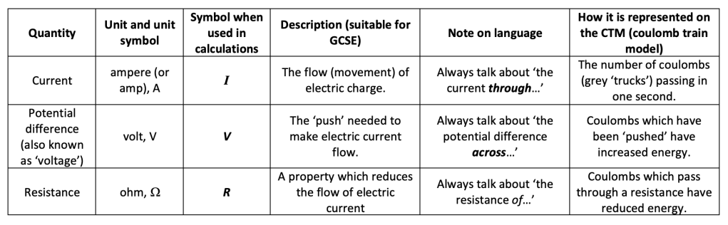
Five coulombs pass through the ammeter in 20 seconds so the current I = Q/t = 5/20 = 0.25 amperes.

Let’s assume we have a 1.5 V cell so 1.5 joules of energy are added to each coulomb as they pass through the cell. Let’s also assume that we have negligible resistance in the cell and the connecting wires so 1.5 joules of energy will be removed from each coulomb as they pass through the resistor. The voltmeter as shown will read 1.5 volts.

The resistance of the resistor R1 is R=V/I = 1.5/0.25 = 6.0 ohms.

---

Let’s Go Parallel First — for real this time.

Now let’s close switch S.

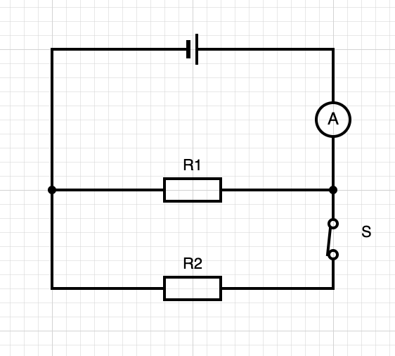
This is example of changing an example by continuous conversion which removes the need for multiple ammeters in the circuit. The changed circuit can be represented on the CTM as shown

Now, ten coulombs pass through the ammeter in twenty seconds so I = Q/t = 10/20 = 0.5 amperes (double the reading in the first circuit shown).

Questioning may be useful at this point to reinforce the ‘flow’ paradigm that we hope students will be using:

• What will be the reading if the ammeter moved to a similar position on the other side? (0.5 amps since current is not ‘used up’.)
• What would be the reading if the ammeter was placed just before resistor R1? (0.25 amps since only half the current goes through R1.)

To calculate the total resistance of the whole circuit we use R = V/I = 1.5/0.5 = 3.0 ohms– which is half of the value of the circuit with just R1. Adding resistors in parallel has the surprising result of reducing the total resistance of the circuit.

This is a concrete example which helps students understand the concept of resistance as a property which reduces current: the current is larger when a second resistor is added so the total resistance must be smaller. Students often struggle with the idea of inverse relationships (i.e. as x increases y decreases and vice versa) so this is a point well worth emphasising.

---

Potential Difference and Parallel Circuits (1)

Let’s expand on the primitive ‘flow’ model we have been using until now and adapt the circuit a little bit.

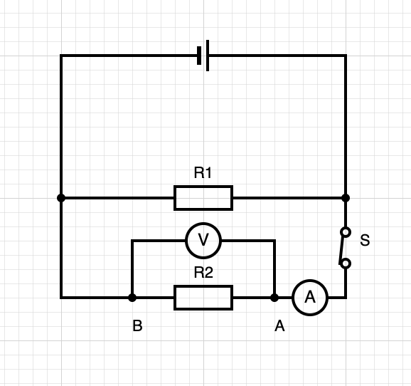
This can be represented on the CTM like this:

Each coulomb passing through R2 loses 1.5 joules of energy so the voltmeter would read 1.5 volts.

One other point worth making is that the resistance of R2 (and R1) individually is still R = V/I = 1.5/0.25 = 6.0 ohms: it is only the combined effect of R1 and R2 together in parallel that reduces the total resistance of the circuit.

---

Potential Difference and Parallel Circuits (2)

Let’s have one last look at a different aspect of this circuit.

This can be represented on the CTM like this:

Each coulomb passing through the cell from X to Y gains 1.5 joules of energy, so the voltmeter would read 1.5 volts.

However, since we have twice the number of coulombs passing through the cell as when switch S is open, then the cell has to load twice as many coulombs with 1.5 joules in the same time.

This means that, although the potential difference is still 1.5 volts, the cell is working twice as hard.

The result of this is that the cell’s chemical energy store will be depleted more quickly when switch S is closed: parallel circuits will make cells go ‘flat’ in a much shorter time compared with a similar series circuit.

Bulbs in parallel may shine brighter (at least in terms of total brightness rather than individual brightness) but they won’t burn for as long.

To some ways of thinking, a parallel circuit with two bulbs is very much like burning a candle at both ends…

---

More fun and high jinks with coulomb train model in the next instalment when we will look at series circuits.

You can read part 5 here.

---

Reference

Redish, E. F., & Kuo, E. (2015). Language of physics, language of math: Disciplinary culture and dynamic epistemology. Science & Education, 24(5), 561-590.