There are three things that everyone should know about simple harmonic motion (SHM).
- Firstly, it is simple;
- Secondly, it is harmonic;
- Thirdly, it is a type of motion.
There, my work here is done. H’mmm — it looks like this physics teaching lark is much easier than is generally acknowledged…

[The above joke courtesy of the excellent Blackadder 2 (1986), of course.]
Misconceptions to the left of us, misconceptions to the right of us…
In my opinion, the misconceptions which hamper students’ attempts to understand simple harmonic motion are:
- A shallow understanding of dynamics which does not differentiate between ‘displacement’ ‘velocity’ and ‘acceleration’ but lumps them together as interchangeable flavours of ‘movement’
- The idea that ‘acceleration’ invariably leads to an increase in the magnitude of velocity and that only the materially different ‘deceleration’ (which is exclusively produced by resistive forces such as friction or drag) can result in a decrease.
- Not understanding the positive and negative direction conventions when analysing motion.
All of these misconceptions can, I believe, be helpfully addressed by using a form of dual coding which I outlined in a previous post.

Top Gear presenters: Assemble!

The discussion context which I present is that of a rather strange episode of the motoring programme Top Gear. You have been given the opportunity to win the car of your dreams if — and only if — you can drive it so that it performs SHM (simple harmonic motion) with a period of 30 seconds and an amplitude of 120 m.
This is a fairly reasonable challenge as it would lead to a maximum acceleration of 5.3 m s-2. For reference, a typical production car can go 0-27 m/s in 4.0 s (a = 6.8 m s-2)) but a Tesla Model S can go 0-27 m/s in a scorching 2.28 s (a = 11.8 m s-2). BTW ‘0-27 m/s’ is the SI civilised way of saying 0-60 mph. It can also be an excellent extension activity for students to check the plausibility of this challenge(!)
Timing and the Top Gear SHM Challenge

- At what time should the car reach E on its outward journey to ensure we meet the Top Gear SHM Challenge? (15 s since A to E is half of a full oscillation and T should be 30 seconds according to the challenge)
- At what time should the car reach C? (7.5 s since this is a quarter of a full oscillation.)
All physics teachers, to a greater or lesser degree, labour under the ‘curse of knowledge’. What we think is ‘obvious’ is not always so obvious to the learner. There is an egregiously underappreciated value in making our implicit assumptions and thinking explicit, and I think diagrams like the above are invaluable in this process.
But what is this SHM (of which you speak of so knowledgeably) anyway?
Simple harmonic motion must fulfil two conditions:
- The acceleration must always be directed towards a fixed point.
- The magnitude of the acceleration is directly proportional to its displacement from the fixed point.
In other words:

Let’s look at this definition in terms of our fanciful Top Gear challenge. More to the point, let’s look at the situation when t = 0 s:
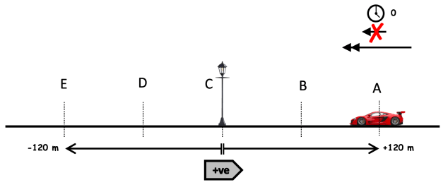
Questions that could be discussed here:
- Why is the displacement at A labelled as ‘+120 m’? (Displacement is a vector and at A it is in the same direction as the [arbitrary] positive direction we have selected and show as the grey arrow labelled +ve.)
- The equation suggests that the value of a should be negative when x is positive. Is the diagram consistent with this? (Yes. The acceleration arrow is directed towards the fixed point C and is in the opposite direction to the positive direction indicated by the grey arrow.)
- What is the value of v indicated on the diagram? Is this consistent with the terms of the challenge? (Zero. Yes, since 120 m is the required amplitude or maximum displacement so if v was greater than zero at this point the car would go beyond 120 m.)
- How could you operate the car controls so as to achieve this part of simple harmonic motion? (You should be depressing the gas pedal to the floor, or ‘pedal to the metal’, to achieve maximum acceleration.)
Model the thinking explicitly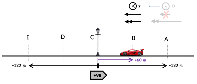
Hands up who thinks the time on the second clock on the diagram above should read 3.75 seconds? It makes sense, doesn’t it? It takes 7.5 s to reach C (one quarter of an oscillation) so the temptation to ‘split the difference’ is nigh on irresistible — except that it would be wrong — and I must confess, it took several revisions of this post before I spotted this error myself (!).
The vehicle is accelerating, so it does not cover equal distances in equal times. It takes longer to travel from A to B than B to C on this part of the journey because the vehicle is gaining speed.
So what is the time when x = 60 m

So we can redraw the diagram as follows:

Some further questions that could be asked are:
- Is the acceleration arrow at B smaller or larger than the acceleration arrow at A? Is this consistent with what we know about SHM? (Smaller. Yes, because for SHM, acceleration is proportional to displacement. The displacement at B is +60 m; the acceleration at B is half the value of the acceleration at A because of this. Note that the magnitude of the acceleration is reduced but the direction of a is still negative since the displacement is positive.)
- Is the velocity at B positive or negative? (Negative, since it is opposite to the positive direction selected on the diagram and shown by the grey ‘+ve’ arrow.)
- Is the magnitude of the velocity at B smaller or larger than at A, and is this consistent with a negative acceleration? (Larger. Yes, since both acceleration and velocity are in the same direction. Note that this is an important point to highlight since many students hold the misconception that a negative acceleration is always a ‘deceleration’.)
- How could you operate the car controls so as to achieve this part of simple harmonic motion? (You should have eased off the gas pedal at this point to achieve half the acceleration obtained at A.)
Next, we move on to this diagram and ask students to use their knowledge of SHM to decide the values of the question marks on the diagram.

Which hopefully should lead to a diagram like the one below, and realisation that at this point, the driver’s foot should be entirely off the gas pedal.

‘Are we there yet?’
And thence to this:

One of the most salient points to highlight in the above diagram is the question: how could you operate the car controls at this point? The answer is of course, that you would be pressing the foot brake pedal to achieve a medium magnitude deceleration. This is often a point of confusion for students: how can a positive acceleration produce a decrease in the magnitude of the velocity? Hopefully, the dual coding convention suggested in this blog post will make this clearer to students.
‘No, really, ARE WE THERE YET?!!’
Nearly.
Over time, we can build up a picture of a complete cycle of SHM, such as the one show below. This shows the car reversing backwards at t = 25 s while the driver gradually increases the pressure on the brake.

From this, it should be easier to relate the results above to graphs of SHM:

A quick check reveals that the displacement is positive and half its maximum value; the acceleration is negative and half of its maximum magnitude; and the velocity is positive and just below its maximum value (since the average deceleration is smaller between C and B than it will be between B and A) .
And finally…
I shall leave the final word to the estimable Top Gear team…

So there you have it: JOB DONE!