e=mc2andallthat

Introduction

The AQA GCSE Required Practical on Acceleration (see pp. 21-22 and pp. 55-57) has proved to be problematic for many teachers, especially those who do not have access to a working set of light gates and data logging equipment.

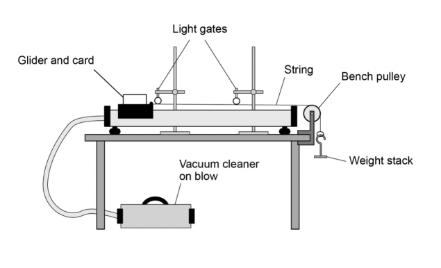
In version 3.8 of the Practical Handbook (pre-March 2018), AQA advised using the following equipment featuring a linear air track (LAT). The “vacuum cleaner set to blow”, (or more likely, a specialised LAT blower), creates a cushion of air that minimises friction between the glider and track.

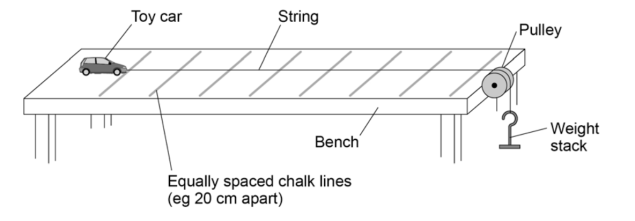
However, in version 5.0 (dated March 2018) of the handbook, AQA put forward a very different method where schools were advised to video the motion of the car using a smartphone in an effort to obtain precise timings at the 20 cm, 40 cm and other marks.

It is possible that AQA published the revised version in response to a number of schools contacting them to say. “We don’t have a linear air track. Or light gates. Or a ‘vacuum cleaner set to blow’.”

The weakness of the “new” version (at least in my opinion) is that it is not quantitative: the method suggested merely records the times at which the toy car passed the lines. Many students may well be able to indirectly deduce the relationship between resultant force and acceleration from this raw timing data; but, to my mind, it would be cognitively less demanding if they were able to compare measurements of resultant force and acceleration instead.

Adapting the AQA method to make it quantitative

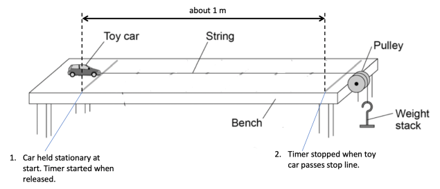
We simplify the AQA method as above: we simply time how long the toy car takes to complete the whole journey from start to finish.

If a runway of one metre or longer is set up, then the total time for the journey of the toy car will be 20 seconds or so for the smallest accelerating weight: this makes manual timing perfectly feasible.

Important note: the length of the runway will be limited by the height of the bench. As soon as the weight stack hits the floor, the toy car will no longer experience an accelerating force and, while it may continue at a constant speed (more or less!) it will no longer be accelerating. In practice, the best way to sort this out is to pull the toy car back so that the weight stack is just below the pulley and mark this position as the start line; then slowly move the toy car forward until the weight stack is just touching the floor, and mark this position as the finish line. Measure the distance between the two lines and this is the length of your runway.

In addition, the weight stack should feature very small masses; that is to say, if you use 100 g masses then the toy car will accelerate very quickly and manual timing will prove to be impossible. In practice, we found that adding small metal washers to an improvised hook made from a paper clip worked well. We found the average mass of the washers by placing ten of them on a scale.

Then input the data into this spreadsheet (click the link to download from Google Drive) and the software should do the rest (including plotting the graph!).

The Eleventh Commandment: Thou Shalt Not Confound Thy Variables!

To confirm the straight line and directly proportional relationship between accelerating force and acceleration, bear in mind that the total mass of the accelerating system must remain constant in order for it to be a “fair test”.

The parts of our system that are accelerating are the toy car, the string and the weight stack. The total mass of the accelerating system shown below is 461 g (assuming the mass of the hook and the string are negligible).

The accelerating (or resultant) force is the weight of 0.2 g mass on the hook, which0 can be calculated using W = mg and will be equal to 0.00196 N or 1.96 mN.

In the second diagram, we have increased the mass on the weight stack to 0.4 g (and the accelerating force to 0.00392 N or 3.92 mN) but note that the total mass of the accelerating system is still the same at 461 g.

In practice, we found that using blu-tac to stick a matchbox tray to the roof of the car made managing and transferring the weight stack easier.

Personal note: as a beginning teacher, I demonstrated the linear air track version of this experiment to an A-level Physics class and ended up disconfirming Newton’s Second Law instead of confirming it; I was both embarrassed and immensely puzzled until an older, wiser colleague pointed out that the variables had been well and truly confounded by not keeping the total mass of the accelerating system constant.

It was embarrassing and that’s why I always harp on about this aspect of the experiment.

What lies beneath: the Physics underlying this method

This can be considered as “deep background” rather than necessary information, but I, for one, consider it really interesting.

Acceleration is the rate of change of a rate of change. Velocity is the rate of change of displacement with time and acceleration is the rate of change of velocity.

Interested individuals may care to delve into higher derivatives like jerk, snap, crackle and pop (I kid you not — these are the technical terms). Jerk is the rate of change of acceleration and hence can be defined as (takes a deep breath) the rate of change of a rate of change of rate of change. More can be found in the fascinating article by Eager, Pendrill and Reistad (2016) linked to above.

But on a much more prosaic level, acceleration can be defined as a = (v – u) / t where v is the final instantaneous velocity, u is the inital instantaneous velocity and t is the time taken for the change.

The instantaneous velocity is the velocity at a momentary instant of time. It is, if you like, the velocity indicated by the needle on a speedometer at a single instant of time and is different from the average velocity which is calculated from the total distance travelled divided the time taken.

This can be shown in diagram form like this:

However, our experiment is simplified because we made sure that the toy car was stationary when the timer was zero; in other words, we ensured u = 0 m/s.

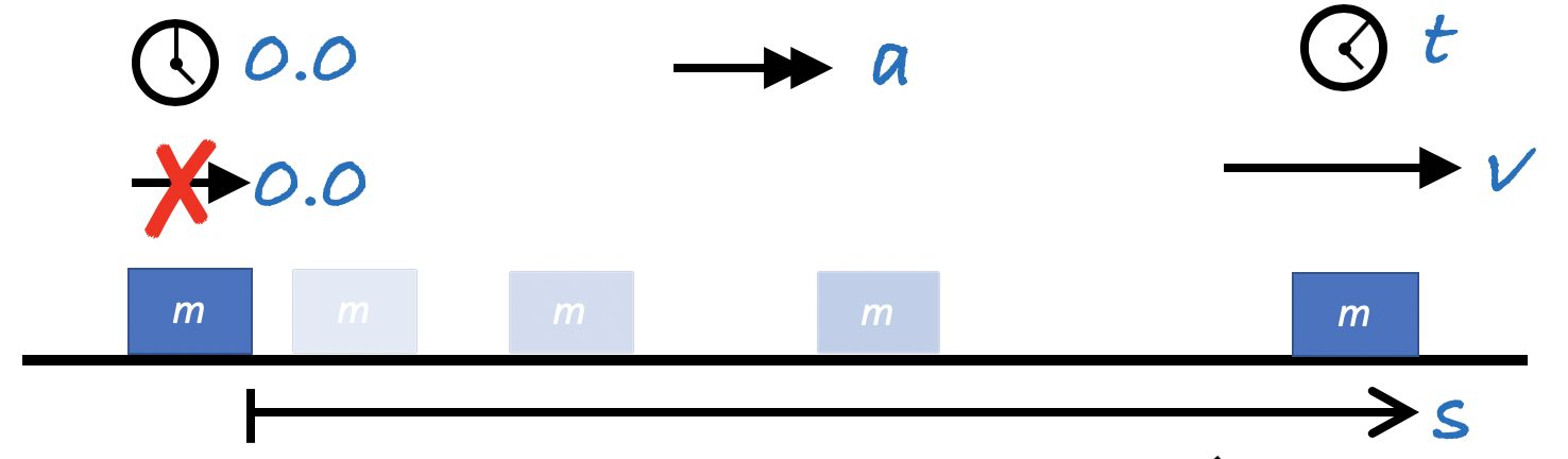
This simplifies a = (v – u) / t to a = v / t.

But how can we find v, the instantaneous velocity at the end of the journey when we have no direct means of measuring it, such as a speedometer or a light gate?

No more jerks left to give

Let’s assume that, for the toy car, the jerk is zero (again, let me emphasize that jerk is a technical term defined as the rate of change of acceleration).

This means that the acceleration is constant.

This fact allows us to calculate the average velocity using a very simple formula: average velocity = (u + v) / t .

But remember that u = 0 so average velocity = v / 2 .

More pertinently for us, provided that u = 0 and jerk = 0, it allows us to calculate a value for v using v = 2 x (average velocity) .

The spreadsheet linked to above uses this formula to calculate v and then uses a = v / t.

Using this in the school laboratory

This could be done as a demonstration or, since only basic equipment is needed, a class experiment. Students may need access to computers running the spreadsheet during the experiment or soon afterwards. We found that one laptop shared between two groups was sufficient.

First experiment (relationship between force and acceleration): set up as shown in the diagram. Place washers totalling a mass of 0.8 g (or similar) and washers totalling a mass of 0.2 g on the hook or weight stack. Hold the toy car stationary at the start line. Release and start the timer. Stop the timer. Input data into the spreadsheet and repeat with different mass on the hook.

It can be useful to get students to manually “check” the value of a calculated by the spreadsheet to provide low stakes practice of using the acceleration formula.

Second experiment (relationship between mass and acceleration). Keep the accelerating force constant with (say) 0.6 g on the hook or weight stack. Hold the toy car stationary at the start line. Release and start the timer. Stop the timer. Input data into the second tab on the spreadsheet and repeat with 100 g added to the toy car (possibly blu-tac’ed into place).

Conclusion

This blog post grew in the telling. Please let me know if you try the methods outlined here and how successful you found them

References

Eager, D., Pendrill, A. M., & Reistad, N. (2016). Beyond velocity and acceleration: jerk, snap and higher derivatives. European Journal of Physics, 37(6), 065008.

Postscript

You can read Part Deux of this blogpost, which details an adaptation of this experiment to work with dynamics trolleys and other standard laboratory equipment.